
In my work with foundry processes, the ability to anticipate the final mechanical properties of a casting before the first mold is poured is a significant advantage. Among these properties, hardness serves as a critical and easily measurable indicator, correlating strongly with tensile strength, yield strength, and the underlying microstructure. For ductile cast iron, the as-cast hardness is predominantly governed by the volume fraction of pearlite in the matrix. While chemical composition, particularly the levels of carbon, silicon, and alloying elements like copper and manganese, sets the foundational potential, the local solid-state cooling conditions within the mold ultimately dictate how this potential is realized. This article details a methodology I have employed, leveraging commercial simulation software, to predict local hardness in ductile cast iron castings by analyzing and correlating simulated cooling rates during the eutectoid transformation.
The metallurgical journey of a ductile cast iron casting from liquid to room temperature involves distinct phase transformations. After solidification, where graphite spheroids are formed within an austenitic matrix, the casting enters the solid-state cooling phase. The most critical segment for determining the final matrix structure is the eutectoid transformation, which typically occurs between approximately 730°C and 780°C. During this transformation, austenite decomposes. The cooling rate through this temperature range is decisive: rapid cooling restricts carbon diffusion, favoring the formation of the fine lamellar mixture of ferrite and cementite known as pearlite. Conversely, slower cooling allows carbon sufficient time to diffuse to existing graphite nodules, resulting in a ferritic matrix surrounding them. Therefore, for a given and controlled chemistry, the local cooling rate during eutectoid transformation becomes the primary variable controlling the pearlite fraction and, consequently, the hardness. This relationship forms the cornerstone of the prediction method.
The core idea is to use casting simulation software, such as MAGMA, not merely for defect analysis but as a quantitative tool to map thermal histories. The software calculates the temperature evolution over time at every node within the virtual casting. By extracting the cooling curve for specific points of interest, one can compute the cooling rate specifically during the eutectoid plateau. This value, calculated as $$V_{cooling} = \frac{\Delta T}{\Delta t}$$ where $\Delta T$ is typically 50°C (from 780°C to 730°C) and $\Delta t$ is the time in minutes to traverse this range, serves as the key predictive parameter. A higher $V_{cooling}$ predicts a higher pearlite fraction and hardness. However, the simulation software’s direct hardness prediction modules can sometimes show significant variance from reality. The proposed method bypasses this by establishing an empirical, casting-specific correlation between the simulated cooling rate and the measured hardness.
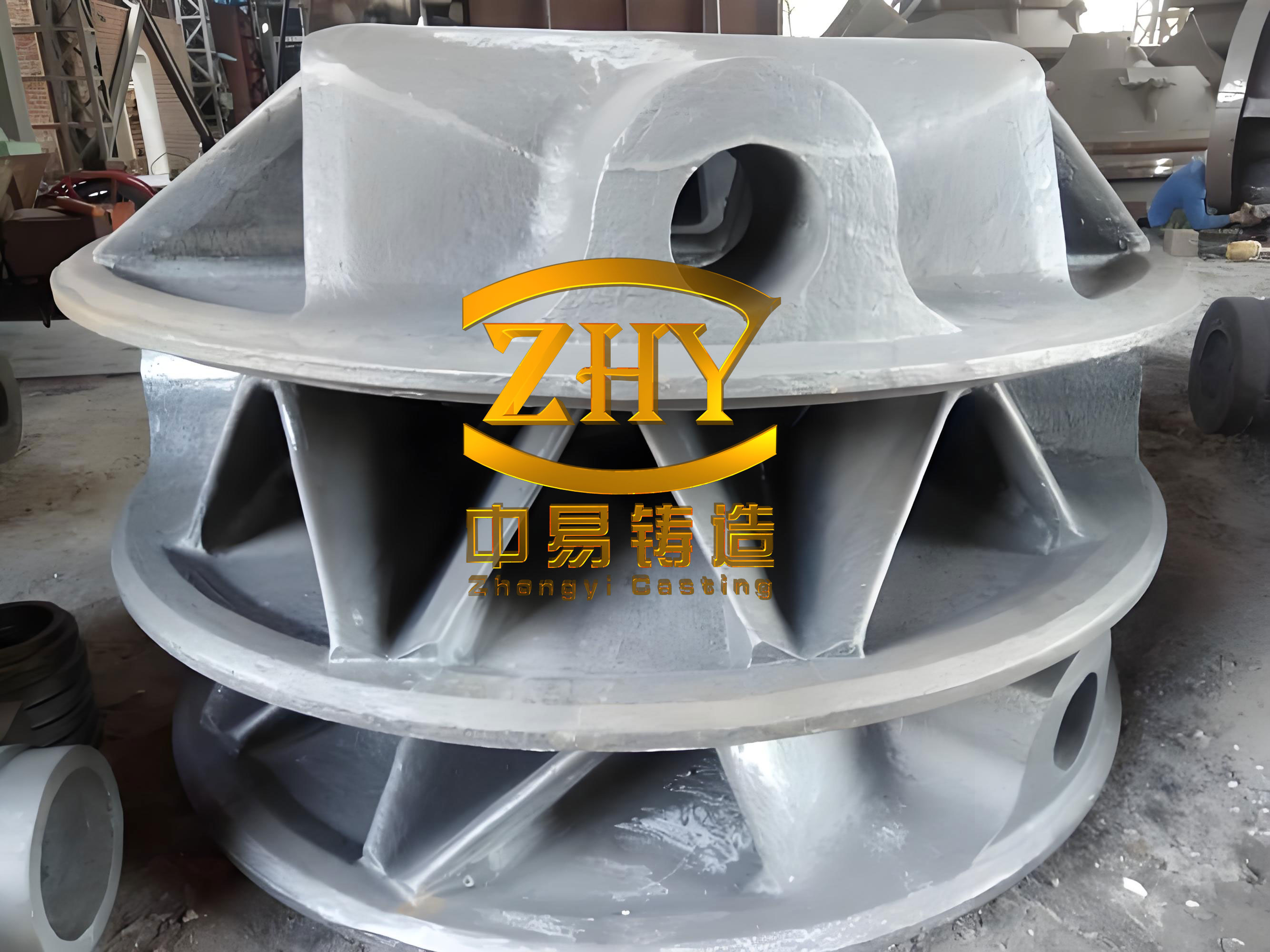
The practical implementation involves a structured validation study. A specific ductile cast iron component with a stable production process is selected. Multiple locations (A, B, C,… M) on the casting are chosen, representing a range of section thicknesses and proximity to feeders or chills. The chemical composition for the trial is tightly controlled, as shown in the example below:
| Element | C | Si | Mn | P | S | Cu | Mg |
|---|---|---|---|---|---|---|---|
| Content (wt.%) | 3.62 | 2.62 | 0.24 | 0.018 | 0.007 | 0.27 | 0.043 |
The process is simulated, and cooling curves for all selected points are exported with high temporal resolution. The cooling rate $V_{cooling}$ for each point is calculated. Subsequently, castings produced under the same conditions are measured for hardness at the corresponding physical locations, ensuring measurements are taken from sufficiently thick sections to ensure accuracy. This generates a dataset pairing simulated cooling rates with actual hardness values (HB).
Analyzing this dataset reveals the empirical correlation. A power-law function often provides a good fit for the relationship between hardness (H) and cooling rate (V). The general form of the equation can be expressed as:
$$H = \alpha \cdot V^{\beta}$$
where $\alpha$ and $\beta$ are constants determined by regression analysis of the experimental data. A more precise model might also incorporate a base hardness influenced by alloy content, but for a fixed chemistry, the power law in $V$ is effective.
For instance, data from a study on a complex casting yielded the following correlations. The central trendline was found to be:
$$H_{mid} = 165.67 \cdot V^{0.0592}$$
To account for natural process variation and measurement scatter, upper and lower bound curves were also established:
$$H_{upper} = 167.72 \cdot V^{0.0602}$$
$$H_{lower} = 161.78 \cdot V^{0.0619}$$
The region between $H_{upper}$ and $H_{lower}$ defines the predicted hardness range for a given cooling rate $V$.
The data from this validation exercise is summarized in the table below, which includes the simulated cooling rate, the average measured hardness, the hardness predicted directly by the software’s internal module (showing sometimes significant error), and the hardness predicted by the empirical cooling-rate model.
| Location | Simulated Cooling Rate, V (ºC/min) | Avg. Measured Hardness (HB) | Software’s Direct Hardness Prediction (HB) | Error of Direct Prediction (%) | Model-Predicted Range (HB) |
|---|---|---|---|---|---|
| A | 8.6 | 190 | 234 | +23.2 | 185-189 |
| B | 33.6 | 202 | 267 | +32.2 | 199-204 |
| C | 18.6 | 195 | 286 | +46.7 | 194-198 |
| D | 19.3 | 190 | 317 | +66.8 | 194-198 |
| E | 18.4 | 193 | 307 | +59.1 | 194-198 |
| F | 15.9 | 197 | 244 | +23.9 | 193-197 |
| G | 53.0 | 211 | 252 | +19.4 | 202-207 |
| H | 23.5 | 197 | 277 | +40.6 | 196-200 |
| I | 19.9 | 204 | 289 | +41.7 | 194-199 |
| J | 23.7 | 200 | 245 | +22.5 | 196-201 |
| K | 32.6 | 208 | 230 | +10.6 | 199-204 |
| L | 13.2 | 196 | 236 | +20.4 | 192-196 |
| M | 14.8 | 193 | 270 | +39.9 | 192-197 |
The true test of the model lies in its predictive capability for a new, unmeasured location (Point N). For the original process, simulation showed a cooling rate $V_N$ = 20.3 ºC/min at Point N. Feeding this value into the empirical correlation model yielded a predicted hardness range of 195-201 HB. The actual measured hardness on the castings was 194 HB, which fell within the predicted band, successfully validating the approach.
Furthermore, the power of this methodology is its utility in process optimization. By modifying the virtual casting process—such as relocating feeders, adding or removing chills, or changing gating geometry—we can simulate the effect on the local cooling rate at a critical point. We then use the established hardness-cooling rate correlation to forecast the outcome. In a follow-up study, five different process modifications were simulated for the same component, all aimed at altering the cooling conditions at Point N while maintaining a nearly identical base chemistry to isolate the thermal effect.
| Process Scheme | Modification Description | Simulated V at N (ºC/min) | Predicted Hardness Range (HB) | Actual Measured Hardness (HB) |
|---|---|---|---|---|
| Original | Baseline layout | 20.3 | 195-201 | 194 |
| Scheme 1 | Removed feeder influence near N | 21.3 | 196-202 | 198 |
| Scheme 2 | Reduced/main runner size, rerouted away from N | 22.0 | 196-202 | 196 |
| Scheme 3 | Further runner modifications | 25.8 | 198-204 | 204 |
| Scheme 4 | Added cooling fins/chills at N | 23.4 | 197-203 | 196 |
| Scheme 5 | Combination of Scheme 2 & 4 | 26.8 | 198-204 | 206 |
The results demonstrate a consistent agreement between the predicted range and the actual measured values. This confirms that the method is not merely descriptive but can be proactively used to engineer the local properties of a ductile cast iron casting by virtually designing the thermal environment.
It is crucial to emphasize that the specific correlation coefficients ($\alpha$, $\beta$) in the power-law model are not universal constants. They are intrinsically tied to the specific context of the study. The actual hardness value is a multivariate function:
$$H = f(V_{cooling}, C_{eq}, [Alloy], Geometry, Sand_type, …)$$
where $C_{eq}$ is the carbon equivalent, $[Alloy]$ represents the specific alloying elements, and other factors include the casting geometry and the cooling properties of the mold medium. The established empirical model works reliably only when all variables except the local cooling rate $V_{cooling}$ are held relatively constant. The correlation must be re-established or recalibrated for a different base chemistry, a significantly different casting family, or a change in molding material (e.g., switching from green sand to resin-bonded sand).
For a more fundamental prediction that accounts for chemistry, one could integrate models for phase transformation kinetics. The fraction of pearlite ($X_p$) can be estimated using an Avrami-type equation adapted for continuous cooling:
$$ X_p = 1 – \exp(-k(T) \cdot t^n) $$
where $k(T)$ is a temperature-dependent rate constant influenced by alloy content, and $t$ is the time spent in the transformation temperature range under a specific cooling profile. The hardness could then be estimated from a linear rule-of-mixtures:
$$ H = X_p \cdot H_{pearlite} + (1 – X_p) \cdot H_{ferrite} + H_{solid-solution} $$
where $H_{pearlite}$ and $H_{ferrite}$ are base hardness values, and $H_{solid-solution}$ accounts for strengthening from dissolved elements like silicon and manganese. While more comprehensive, this approach requires precise material data for the specific ductile cast iron grade.
Based on my experience, I recommend the following practical guide for implementing this hardness prediction method:
- Select a Stable Baseline: Choose a component and a well-controlled, stable production process as your calibration benchmark.
- Define Measurement Grid: Identify 10-15 distinct locations on the casting that cover a wide spectrum of expected cooling conditions (thin walls, thick sections, near feeders, isolated areas).
- Execute Calibration Run: Simulate the standard process and calculate $V_{cooling}$ for each point. Produce castings and meticulously measure hardness at the exact corresponding locations.
- Establish Correlation: Perform regression analysis on the (V, H) data pairs. A power-law fit is a robust starting point. Determine the confidence interval or upper/lower bounds to create a prediction band.
- Validate and Use: Test the correlation by predicting hardness at a few “unknown” points not used in the regression. Then, employ the model to virtually test process changes for achieving desired hardness targets in specific zones.
In conclusion, the integration of casting simulation software with empirical data analysis provides a powerful and practical tool for predicting and controlling the hardness of ductile cast iron castings. By focusing on the simulated cooling rate during the critical eutectoid transformation and establishing a component-specific correlation with measured hardness, foundries can move beyond qualitative defect analysis towards quantitative property engineering. This method significantly reduces the trial-and-error cost and lead time associated with developing robust casting processes, especially for complex components where achieving uniform or specified hardness gradients is essential. While the specific correlation is context-dependent, the underlying principle—linking simulated thermal history to a key mechanical property—is a valuable strategy for advancing the science and reliability of ductile cast iron production.