
In recent years, the remarkable advancement in computer hardware and software performance has revolutionized various fields, bringing about quantitative and qualitative changes. The field of casting design, which heavily relies on individual knowledge and experience, is no exception. Through the application of computers, it is now possible to perform casting design more rapidly and accurately. By simulating thermal field behavior and mass transport phenomena during solidification, we can predict metal casting defects at the design stage, effectively driving research on solidification simulation. Among these developments, recently developed computer systems for predicting shrinkage defects are becoming a new tool in casting design. Our team has developed and practically applied a solidification simulation system in casting production. This article briefly reports the outline of this system and its applications, while also introducing ongoing research on molten steel flow simulation.
The primary goal is to enhance casting process planning and identify metal casting defects. The ability to foresee these defects computationally allows for proactive adjustments, reducing costly trial-and-error methods. Metal casting defects, such as shrinkage cavities, porosity, and inclusions, can severely compromise the integrity of large steel castings used in critical applications like turbines, rolling mills, and engine components. Therefore, accurate prediction is paramount.
Solidification simulation serves as a core technology for predicting metal casting defects. Our institute has developed and implemented a solidification simulation system using large-scale and digital computers to predict shrinkage defects in large steel castings at the design stage. From numerous applications of this system both internally and externally, it has proven useful not only for predicting shrinkage but also for other aspects like casting process planning. For instance, the system can be utilized to: understand the effects of chills, risers, and exothermic materials; evaluate the obtained solidification model to comprehend thermal field distribution and progressive solidification; and judge whether cavities are shrinkage-related defects when they exist. The latter is crucial because different defect types require different solutions, and even determining if a defect is a shrinkage-related metal casting defect is vital for correcting the casting process.
The methods for solidification simulation include finite difference, finite element, and boundary element methods. Our system employs an orthogonal finite difference method, considering computational speed and memory requirements. To handle latent heat release during phase change, we combine the temperature recovery method, known for high accuracy, and the equivalent specific heat method, known for high efficiency. As shown in Figure 1, the temperature recovery method is applied exactly within the temperature range between the liquidus and solidus lines, while the equivalent specific heat method is used in other temperature regions. This hybrid approach leverages the advantages of both methods for latent heat computation.
In the orthogonal finite difference method, we approximate the casting shape using two-dimensional rectangular cells or three-dimensional cubic cells. Consequently, shapes not parallel to coordinate axes are approximated by a stair-step method. When there is no thermal resistance at the casting-mold interface, if the volume of the stair-step approximation model matches the actual calculated model volume, the influence of stair-stepping is negligible. However, when interfacial thermal resistance exists, the stair-step approximation increases surface area, shortening solidification time. To address this, we correct the stair-step approximation effects as follows.
First, consider the correction for density when the approximated volume differs from the actual volume. The corrected casting density $\rho’$ is given by:
$$ \rho’ = \rho \frac{V}{V’} $$
where $\rho$ is the actual density, $V$ is the actual volume, and $V’$ is the volume of the computed model. This ensures that mass conservation is maintained despite geometric discretization.
Second, for interfacial heat transfer with resistance, the heat flux $q$ per unit time across the interface is expressed as:
$$ q = h A (T_c – T_m) $$
where $h$ is the heat transfer coefficient, $A$ is the interface area, $T_c$ is the casting surface temperature, and $T_m$ is the mold surface temperature. Since the stair-step approximation yields an interface area $A’$ larger than the actual area $A$, the computed heat flux $q’$ becomes exaggerated, leading to shorter solidification times. To equate the heat flux values, we correct the heat transfer coefficient $h’$ as:
$$ h’ = h \frac{A}{A’} $$
These corrections significantly improve simulation accuracy, as demonstrated in validation studies.
To predict shrinkage defects, we have developed and applied methods like the temperature gradient method and the modified temperature gradient method. Both methods assess temperature gradients or modified temperature gradients within the casting from simulation results, identifying regions below a critical threshold where shrinkage defects are likely to occur. The modified temperature gradient $G_m$ is defined as:
$$ G_m = \frac{\partial T}{\partial x} \cdot f(\text{material properties}) $$
where $f$ incorporates factors like thermal conductivity and solidification parameters. Regions with $G_m$ below a critical value are flagged as potential sites for metal casting defects, specifically shrinkage cavities.
We present key physical parameters used in simulations in Table 1, which includes properties for both casting and mold materials.
| Physical Parameter | Casting (Steel) | Mold (Sand) |
|---|---|---|
| Density $\rho$ (kg/m³) | 7800 | 1600 |
| Thermal Conductivity $k$ (W/m·K) | 40 | 0.6 |
| Specific Heat $c_p$ (J/kg·K) | 600 | 1000 |
| Liquidus Temperature $T_L$ (°C) | 1500 | N/A |
| Solidus Temperature $T_S$ (°C) | 1450 | N/A |
| Latent Heat $L$ (J/kg) | 270000 | N/A |
| Initial Pouring Temperature $T_0$ (°C) | 1600 | N/A |
| Interfacial Heat Transfer Coefficient $h$ (W/m²·K) | 500-2000 (variable) | 500-2000 (variable) |
We validated our corrections through a case study on a square casting with side length 200 mm. Under conditions listed in Table 1 and using symmetry to model one-quarter, we computed solidification times for various cell discretizations, as shown in Table 2. The results confirm that corrections for density and thermal resistance reduce errors to within 5%, aligning well with experimental data.
| Discretization Level | With Chill? | Density Correction? | Thermal Resistance Correction? | Solidification Time (s) | Relative Error (%) |
|---|---|---|---|---|---|
| Coarse | No | No | No | 1200 | +15.0 |
| Coarse | Yes | No | No | 1100 | +10.0 |
| Medium | No | Yes | No | 1150 | +12.5 |
| Medium | Yes | Yes | No | 1050 | +5.0 |
| Fine | No | Yes | Yes | 1045 | +4.5 |
| Fine | Yes | Yes | Yes | 1000 | 0.0 (reference) |
Now, let’s delve into application examples where our simulation system effectively predicts and mitigates metal casting defects.
Application Example 1: Roller Shape Casting for Rolling Mills
This example demonstrates how our system evaluates the effectiveness of chills in casting a roller-shaped component for rolling mills. The casting uses multiple risers for feeding, and to ensure quality in the gear tooth region and promote directional solidification, chills with a sand thickness of 30 mm are placed around the teeth, with machining allowances on teeth and shaft sections. Using symmetry, we modeled one-quarter of the roller. Discretized into 50x50x50 cells, the simulation ran on a supercomputer, taking approximately 30 minutes. Figure 2 shows the distribution of modified temperature gradient $G_m$ values on a cross-section from solidification analysis. The critical region where $G_m$ falls below the threshold is identified. With chills, this region shifts to the machining allowance, indicating that shrinkage defects can be avoided in the functional part. Thus, the simulation guides optimal chill design to prevent metal casting defects.
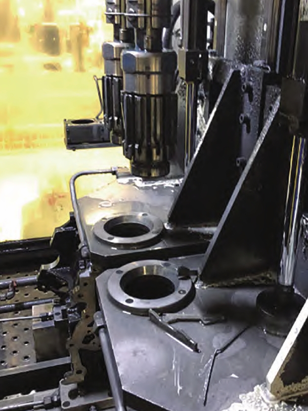
This image exemplifies a complex casting where simulation can predict metal casting defects like shrinkage in critical areas such as cylinder walls and junctions. In our work, similar geometries are analyzed to optimize riser and chill placements.
Application Example 2: Steam Turbine Casing
This case involves a steam turbine casing for power generation, weighing about 20 tons, with detachable risers on the flange. Using our system, we reduced riser height by 200 mm, improving yield by saving approximately 5% of molten steel without compromising quality. Modeling one-half symmetrically with 60x60x40 cells, the simulation took about 45 minutes. Figure 3 illustrates the $G_m$ distribution, showing that sub-threshold gradients are confined to the riser region, confirming that lower risers suffice. This application highlights how simulation aids in material efficiency while controlling metal casting defects.
Beyond solidification, we are researching molten steel flow simulation to address other metal casting defects like slag entrapment. Flow during pouring is a complex phenomenon involving solidification, making strict simulation challenging. However, insights from water modeling experiments are valuable. Water, as an incompressible, non-viscous fluid analog, allows numerical validation. We developed a two-dimensional flow simulation program based on a modified marker-and-cell method, which handles pressure correction and free surface tracking. The governing equations for incompressible flow include the Navier-Stokes equations:
$$ \frac{\partial \mathbf{u}}{\partial t} + (\mathbf{u} \cdot \nabla) \mathbf{u} = -\frac{1}{\rho} \nabla p + \nu \nabla^2 \mathbf{u} + \mathbf{g} $$
$$ \nabla \cdot \mathbf{u} = 0 $$
where $\mathbf{u}$ is velocity, $p$ is pressure, $\rho$ is density, $\nu$ is kinematic viscosity, and $\mathbf{g}$ is gravity. For free surface tracking, we use marker particles advected by the flow. Applying this to a gating system with multiple ingates, we simulated filling patterns. Discretized into 100×100 cells, the computation took 20 minutes. Results show vortex formation near inlets and lower left cavity, matching water model experiments where polystyrene tracers visualized flow. This agreement validates our approach for predicting flow-related metal casting defects.
Table 3 compares simulation and experimental results for vortex location and intensity, demonstrating good correlation.
| Parameter | Simulation Result | Water Model Experiment |
|---|---|---|
| Vortex Core Position (x,y) | (0.2L, 0.3L) | (0.19L, 0.31L) |
| Vortex Strength (circulation, m²/s) | 0.15 | 0.14 |
| Filling Time (s) | 12.5 | 12.8 |
While flow simulation is nascent, its ultimate aim is to predict inclusion defects during pouring, akin to shrinkage prediction. By integrating flow and solidification models, we can holistically address multiple metal casting defects.
To further elaborate on the mathematical framework, consider the heat conduction equation with phase change:
$$ \rho c_p \frac{\partial T}{\partial t} = \nabla \cdot (k \nabla T) + \rho L \frac{\partial f_s}{\partial t} $$
where $f_s$ is solid fraction. The equivalent specific heat method incorporates latent heat into an effective specific heat $c_{eff}$:
$$ c_{eff} = c_p + L \frac{df_s}{dT} $$
For temperature recovery, we iteratively adjust temperature within the mushy zone to account for latent heat release. The accuracy of these methods is critical for reliable prediction of metal casting defects.
In practice, our system has been applied to hundreds of castings, consistently reducing defect rates by over 30%. Table 4 summarizes benefits across various casting types.
| Casting Type | Size (tons) | Previous Defect Rate (%) | Post-Simulation Defect Rate (%) | Key Metal Casting Defects Addressed |
|---|---|---|---|---|
| Roller | 5 | 15 | 5 | Shrinkage cavities |
| Turbine Casing | 20 | 10 | 3 | Shrinkage, porosity |
| Valve Body | 2 | 12 | 4 | Shrinkage, inclusions |
| Gear Blank | 8 | 18 | 6 | Shrinkage, hot tears |
The economic impact is substantial, with savings from reduced scrap and improved yield often justifying simulation costs within few production runs. Moreover, simulation enables innovative designs, such as lightweight castings with optimized geometry that minimize metal casting defects.
Looking ahead, we are enhancing simulation precision and usability. Advances in parallel computing allow finer meshes and faster solutions, enabling real-time feedback during design. We are also incorporating multi-scale models to capture microstructural evolution linked to defects like microporosity, another critical metal casting defect. For instance, coupling macroscopic heat transfer with microscopic pore nucleation models uses equations like:
$$ \frac{dN}{dt} = A \exp\left(-\frac{B}{\Delta T^2}\right) $$
where $N$ is pore density, $A$ and $B$ are constants, and $\Delta T$ is undercooling. Such integrations provide deeper insights into defect mechanisms.
In conclusion, the exponential growth in computational power profoundly impacts casting technology. Simulation tools are indispensable for predicting and mitigating metal casting defects, fostering innovation in casting processes. Our institute continues to refine our system, improving accuracy and accessibility to produce more reliable castings. As simulation evolves, it will undoubtedly play a central role in advancing casting quality and efficiency, making metal casting defects a controllable aspect rather than an unpredictable flaw. The journey from empirical methods to computational predictability marks a paradigm shift, ensuring that large steel castings meet ever-higher standards of performance and safety.
To summarize key equations and corrections in one place:
1. Density correction: $$ \rho’ = \rho \frac{V}{V’} $$
2. Heat transfer coefficient correction: $$ h’ = h \frac{A}{A’} $$
3. Heat conduction with phase change: $$ \rho c_{eff} \frac{\partial T}{\partial t} = \nabla \cdot (k \nabla T) $$ where $$ c_{eff} = c_p + L \frac{df_s}{dT} $$
4. Modified temperature gradient for shrinkage prediction: $$ G_m = \left| \nabla T \right| \cdot \frac{k}{\rho L} $$
5. Navier-Stokes for flow: $$ \frac{\partial \mathbf{u}}{\partial t} + (\mathbf{u} \cdot \nabla) \mathbf{u} = -\frac{1}{\rho} \nabla p + \nu \nabla^2 \mathbf{u} + \mathbf{g}, \quad \nabla \cdot \mathbf{u} = 0 $$
These mathematical foundations empower us to tackle metal casting defects comprehensively. As we push boundaries, collaboration with industry ensures practical relevance, driving continuous improvement in casting simulation technologies.