
1. Introduction
In the modern manufacturing industry, the demand for automation and intelligence in production processes is continuously increasing. Among various processing stages, flash grinding plays a crucial role in determining the surface quality and aesthetic appearance of steel castings. Traditional manual grinding is not only inefficient but also poses significant safety risks to workers. The dusty and noisy environment, combined with high labor intensity, makes manual grinding an undesirable option for large-scale production. To address these challenges, many manufacturers are turning to robotic grinding systems that integrate advanced sensor technologies, computer vision, and robot control algorithms. In this thesis, I focus on the automatic detection of flashes on steel castings and the planning of grinding paths using three-dimensional point cloud processing techniques combined with robot trajectory generation methods. The proposed workflow enables a robot to follow a precisely generated trajectory to remove flashes efficiently and accurately, thereby improving productivity and product quality.
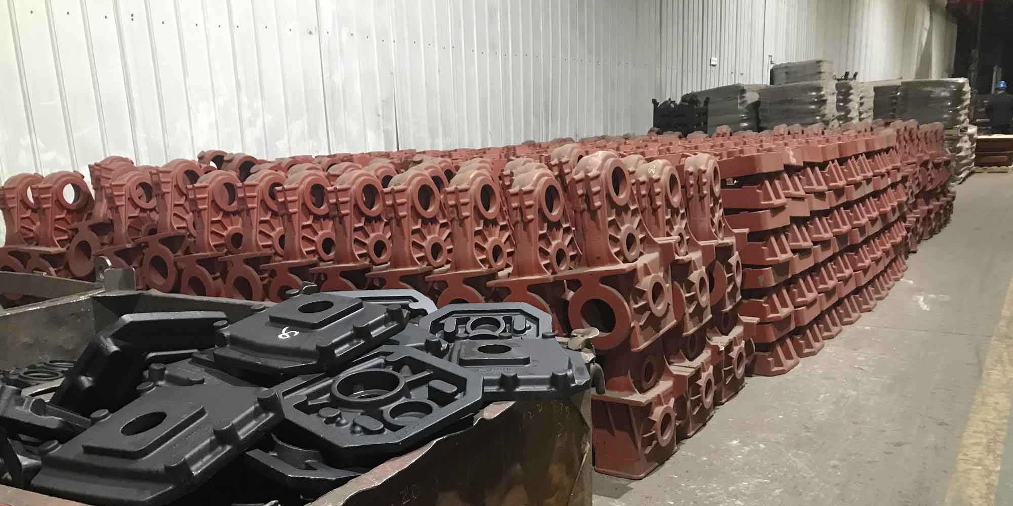
The research presented in this thesis addresses three key challenges in robotic flash grinding: (1) accurate pose estimation of steel castings from point cloud data, (2) robust detection and segmentation of flash regions, and (3) generation of smooth and precise robot trajectories based on the extracted flash contours. I propose a point cloud registration algorithm based on principal component analysis (PCA) and normal vector constraints to achieve high-accuracy pose estimation even when the initial positions of the scanned and reference point clouds are significantly different. For flash detection, I combine alpha shapes boundary extraction with an improved voxel-grid downsampling method to obtain a clean set of path points. Finally, I design a fifth-degree non-uniform B-spline interpolation algorithm that generates a smooth curve passing through all the desired grinding points, enabling the robot to perform continuous and stable motions.
This thesis is organized as follows. Section 2 describes the grinding process, workpiece characteristics, coordinate transformation models, and robot kinematics. Section 3 presents the point cloud preprocessing, registration, and segmentation algorithms for flash region detection. Section 4 discusses trajectory planning methods and introduces the proposed spline interpolation algorithm. Section 5 describes the developed point cloud processing system and experimental verification. Section 6 concludes the thesis and discusses future work.
2. Grinding Process and System Design
2.1 Flash Characteristics and Grinding Workflow
Steel castings are produced by pouring molten metal into molds. Due to gaps between mold halves, improper mold design, or poor filling quality, excess material known as flashes or burrs often appears on the edges, corners, and hole boundaries of the castings. These flashes affect the dimensional accuracy and surface roughness of the final product. Therefore, grinding is necessary to smooth the surface and bring the casting within the specified tolerances.
In a typical manufacturing environment, the grinding of steel castings is performed manually, which is labor-intensive and hazardous. To replace manual operations, I propose an automated workflow that integrates a 3D laser scanner, a six-axis industrial robot, and a controller. The workflow is illustrated as a sequence of steps:
- Fix the steel casting on a worktable.
- Scan the casting using a 3D laser scanner to acquire raw point cloud data.
- Transmit the point cloud to a client computer.
- Preprocess the point cloud to remove noise and downsample while preserving features.
- Register the scanned point cloud with a standard CAD model to determine the exact pose.
- Segment the flash regions and extract grinding path points.
- Generate a smooth robot trajectory using spline interpolation.
- Send the trajectory to the robot controller to execute the grinding process.
This workflow reduces human intervention and improves consistency, as the robot can repeatedly perform grinding operations with high precision.
2.2 Coordinate System Transformation
To coordinate the robot, the scanner, and the casting, I define multiple coordinate systems: the robot base frame \(\{B\}\), the flange frame \(\{E\}\), the tool frame \(\{T\}\), the worktable frame \(\{W\}\), the casting frame \(\{C\}\), and the laser scanner frame \(\{M\}\). The relationships among these frames are described by homogeneous transformation matrices. For any point \(\mathbf{p}\) expressed in a frame \(\{A\}\), its coordinates in another frame \(\{B\}\) are obtained by:
$$
\begin{bmatrix} \mathbf{p}_B \\ 1 \end{bmatrix} = \mathbf{T}_{AB} \begin{bmatrix} \mathbf{p}_A \\ 1 \end{bmatrix}
$$
where \(\mathbf{T}_{AB}\) is the \(4\times4\) homogeneous transformation matrix:
$$
\mathbf{T}_{AB} = \begin{bmatrix} \mathbf{R}_{AB} & \mathbf{t}_{AB} \\ \mathbf{0}^T & 1 \end{bmatrix}
$$
Here, \(\mathbf{R}_{AB}\) is a \(3\times3\) rotation matrix and \(\mathbf{t}_{AB}\) is a translation vector. By composing the transformations from the robot base to the scanner and from the scanner to the casting, I can determine the casting’s position in the robot base frame. This transformation chain is essential for guiding the robot to the correct grinding locations.
2.3 Robot Kinematic Model
I adopt the Denavit-Hartenberg (D-H) convention to model the six-degree-of-freedom (6-DOF) robot. Each link coordinate frame is established according to the D-H parameters. The transformation between adjacent links \(i-1\) and \(i\) is:
$$
\mathbf{T}_i^{i-1} = \begin{bmatrix} \cos\theta_i & -\sin\theta_i \cos\alpha_{i-1} & \sin\theta_i \sin\alpha_{i-1} & a_{i-1} \cos\theta_i \\ \sin\theta_i & \cos\theta_i \cos\alpha_{i-1} & -\cos\theta_i \sin\alpha_{i-1} & a_{i-1} \sin\theta_i \\ 0 & \sin\alpha_{i-1} & \cos\alpha_{i-1} & d_i \\ 0 & 0 & 0 & 1 \end{bmatrix}
$$
The D-H parameters of the 6-DOF robot used in this work are listed in the following table:
| Link \(i\) | \(\alpha_{i-1}\) (rad) | \(a_{i-1}\) (mm) | \(d_i\) (mm) | \(\theta_i\) (deg) |
|---|---|---|---|---|
| 1 | \(-\pi/2\) | 0 | 0 | \(\theta_1\) |
| 2 | 0 | \(a_2\) | 0 | \(\theta_2\) |
| 3 | \(-\pi/2\) | \(a_3\) | \(d_3\) | \(\theta_3\) |
| 4 | \(\pi/2\) | 0 | \(d_4\) | \(\theta_4\) |
| 5 | \(-\pi/2\) | 0 | 0 | \(\theta_5\) |
| 6 | 0 | 0 | 0 | \(\theta_6\) |
The forward kinematics are obtained by multiplying the individual link transformation matrices:
$$
\mathbf{T}_6^0 = \mathbf{T}_1^0 \mathbf{T}_2^1 \mathbf{T}_3^2 \mathbf{T}_4^3 \mathbf{T}_5^4 \mathbf{T}_6^5 = \begin{bmatrix} n_x & s_x & a_x & p_x \\ n_y & s_y & a_y & p_y \\ n_z & s_z & a_z & p_z \\ 0 & 0 & 0 & 1 \end{bmatrix}
$$
The inverse kinematics solution is derived using an analytic approach based on the relationship between the desired end-effector pose and the joint variables. The Jacobian matrix \(\mathbf{J}\) relates the end-effector velocity to the joint velocities:
$$
\begin{bmatrix} \dot{x} \\ \dot{y} \\ \dot{z} \end{bmatrix} = \mathbf{J} \begin{bmatrix} \dot{\theta}_1 \\ \dot{\theta}_2 \\ \dot{\theta}_3 \\ \dot{\theta}_4 \\ \dot{\theta}_5 \\ \dot{\theta}_6 \end{bmatrix}
$$
The Jacobian is also used for redundancy resolution and singularity analysis, which are important for ensuring smooth trajectory tracking.
2.4 Simulation System Architecture
I built a simulation environment for the steel casting grinding system using SOLIDWORKS for modeling and MATLAB for kinematic analysis. The system includes a 6-axis industrial robot model, a worktable, and a steel casting model with flashes. The robot workspace was analyzed using the Monte Carlo method. By randomly sampling joint angles within their limits and computing the forward kinematics, I obtained a cloud of reachable end-effector positions. The workspace approximates a sphere with a radius of about 1000 mm, which is sufficient for the casting sizes considered in this study. This simulation system allows me to verify the algorithm-generated trajectories before actual deployment.
3. Flash Region Detection on Steel Castings
3.1 Point Cloud Preprocessing
The raw point cloud data acquired from the scanner often contains noise, outliers, and redundant points. To improve the efficiency and accuracy of subsequent processing, I apply a voxel-grid downsampling method to reduce the point density while retaining the essential geometric features. For each voxel, the centroid of the points inside is computed as:
$$
x_c = \frac{1}{n}\sum_{i=1}^{n} x_i, \quad y_c = \frac{1}{n}\sum_{i=1}^{n} y_i, \quad z_c = \frac{1}{n}\sum_{i=1}^{n} z_i
$$
After downsampling, I extract feature points based on normal vector variation. For each point \(\mathbf{p}_i\), I search its \(k\) nearest neighbors using a k-d tree. The mean angle between the normal vector of \(\mathbf{p}_i\) and the normals of its neighbors is calculated as:
$$
\gamma_i = \frac{1}{k} \sum_{j=1}^{k} \theta_{ij}
$$
where \(\theta_{ij}\) is the angle between the normal of point \(i\) and that of its \(j\)-th neighbor. Points with a large \(\gamma_i\) are retained as feature points, as they indicate high curvature regions likely to contain flashes or edges. This step significantly reduces the number of points while preserving important shape details.
3.2 Steel Casting Pose Estimation
3.2.1 Principal Component Analysis for Axis Alignment
To improve the robustness of point cloud registration, I first align the principal axes of the source and target point clouds using PCA. For a point cloud set \(P = \{\mathbf{p}_i\}_{i=1}^{N}\), the covariance matrix is:
$$
\mathbf{C}_P = \frac{1}{N} \sum_{i=1}^{N} (\mathbf{p}_i – \bar{\mathbf{p}})(\mathbf{p}_i – \bar{\mathbf{p}})^T
$$
where \(\bar{\mathbf{p}} = \frac{1}{N}\sum_{i=1}^{N}\mathbf{p}_i\) is the centroid. The eigenvectors of \(\mathbf{C}_P\) constitute an orthonormal frame representing the principal directions. Similarly, the covariance matrix \(\mathbf{C}_Q\) is computed for the target point cloud \(Q\). The rotation matrix that aligns the two frames is:
$$
\mathbf{R}_0 = \mathbf{V}_P \mathbf{V}_Q^{-1}
$$
and the translation vector is \(\mathbf{t}_0 = \bar{\mathbf{q}} – \mathbf{R}_0 \bar{\mathbf{p}}\). Because the eigenvectors may be oriented in opposite directions, there are eight possible axis alignments. I evaluate all eight cases and select the one that minimizes the mean squared error between the transformed source and the target. This provides a good initial alignment for the subsequent registration steps.
3.2.2 Four-Point Congruent Sets (4PCS) for Global Registration
After principal axis alignment, I apply the 4PCS algorithm to perform coarse registration. 4PCS is a global registration method that is robust to noise and low overlap. The algorithm selects four coplanar points in the source point cloud with a large spatial extent and computes their affine invariant ratios. These ratios are then used to find corresponding four-point sets in the target cloud. For each candidate set, a transformation is estimated and the one with the largest common point set (LCP) score is chosen. The coarse registration provides an improved initial pose for the fine registration stage.
3.2.3 Improved ICP with Normal Vector Constraints
For fine registration, I improve the classical Iterative Closest Point (ICP) algorithm by incorporating normal vector constraints and a bidirectional k-d tree search. The steps are as follows:
- Compute the normals of both point clouds using local surface fitting.
- For each point in the source cloud, find the nearest neighbor in the target cloud using a k-d tree, but only accept pairs whose distance is below a threshold.
- Additionally, reject pairs if the angle between their normal vectors is greater than a threshold \(\tau\). This removes many incorrect correspondences.
- Calculate the transformation \((\mathbf{R}, \mathbf{t})\) that minimizes the error function:
$$
E(\mathbf{R}, \mathbf{t}) = \frac{1}{n} \sum_{i=1}^{n} \left\| \mathbf{q}_i – (\mathbf{R} \mathbf{p}_i + \mathbf{t}) \right\|^2
$$
- Iterate until convergence, i.e., the change in error between successive iterations is below a small threshold or a maximum number of iterations is reached.
This improved ICP greatly accelerates convergence and avoids local minima, especially when the initial pose is not very accurate. The final transformation matrix gives the exact pose of the scanned steel casting relative to the reference model.
3.2.4 Registration Performance Evaluation
To validate the proposed registration algorithm, I conducted experiments on three public point cloud datasets (Bunny, Dragon, Armadillo) and three steel casting point clouds. The comparative results with other methods are summarized in the following tables.
| Dataset | Method | RMSE (m) | Time (s) |
|---|---|---|---|
| Bunny | SAC-IA+NDT | \(4.03\times10^{-5}\) | 4.193 |
| ISS+3DSC+ICP | \(2.13\times10^{-5}\) | 4.138 | |
| NDT+ICP | \(3.13\times10^{-5}\) | 2.923 | |
| Ours | \(\mathbf{0.32\times10^{-6}}\) | \(\mathbf{0.598}\) | |
| Dragon | SAC-IA+NDT | \(3.61\times10^{-5}\) | 6.072 |
| ISS+3DSC+ICP | \(3.16\times10^{-5}\) | 5.036 | |
| NDT+ICP | \(5.12\times10^{-5}\) | 5.313 | |
| Ours | \(\mathbf{0.36\times10^{-6}}\) | \(\mathbf{0.831}\) | |
| Armadillo | SAC-IA+NDT | \(3.13\times10^{-5}\) | 5.215 |
| ISS+3DSC+ICP | \(3.17\times10^{-5}\) | 5.836 | |
| NDT+ICP | \(3.11\times10^{-5}\) | 4.724 | |
| Ours | \(\mathbf{0.17\times10^{-6}}\) | \(\mathbf{0.766}\) |
| Point cloud set | Method | RMSE (m) | Time (s) |
|---|---|---|---|
| Set 1 | SAC-IA+NDT | \(3.15\times10^{-5}\) | 3.28 |
| ISS+3DSC+ICP | \(2.23\times10^{-5}\) | 2.53 | |
| NDT+ICP | \(2.58\times10^{-5}\) | 2.38 | |
| Ours | \(\mathbf{0.53\times10^{-6}}\) | \(\mathbf{0.86}\) | |
| Set 2 | SAC-IA+NDT | \(3.53\times10^{-5}\) | 5.15 |
| ISS+3DSC+ICP | \(3.56\times10^{-5}\) | 4.87 | |
| NDT+ICP | \(6.95\times10^{-5}\) | 6.36 | |
| Ours | \(\mathbf{0.78\times10^{-6}}\) | \(\mathbf{0.71}\) | |
| Set 3 | SAC-IA+NDT | \(4.36\times10^{-5}\) | 4.57 |
| ISS+3DSC+ICP | \(5.52\times10^{-5}\) | 5.73 | |
| NDT+ICP | \(3.73\times10^{-5}\) | 5.02 | |
| Ours | \(\mathbf{0.49\times10^{-6}}\) | \(\mathbf{0.91}\) |
The results demonstrate that the proposed method achieves sub-micrometer accuracy and completes the registration in less than one second, outperforming other state-of-the-art approaches in both accuracy and efficiency.
3.3 Flash Edge Extraction Using Alpha Shapes
Once the steel casting point cloud is accurately registered, I need to identify the flash regions that require grinding. The flash is typically located on the edges of the casting or around holes. I first segment the flash points from the main body by comparing the scanned point cloud with the standard model. Using a k-d tree, I mark points in the scanned cloud that are within a certain distance from the standard model as belonging to the body; the remaining points are considered flash points.
To extract the boundary of the flash region, I apply the alpha shapes algorithm. The alpha shapes method constructs a geometric shape around a point set using a parameter \(\alpha\), which controls the level of detail. For a set of points, the boundary edges are determined by rolling a circle of radius \(\alpha\) around the point set. A point is deemed a boundary point if the circle does not contain any other points. The center of a candidate circle for two points \(\mathbf{p}_1(x_1,y_1)\) and \(\mathbf{p}_2(x_2,y_2)\) can be computed as:
$$
x_0 = x_1 + \frac{1}{2}(x_2 – x_1) – h(y_2 – y_1)
$$
$$
y_0 = y_1 + \frac{1}{2}(y_2 – y_1) + h(x_2 – x_1)
$$
where
$$
h = \sqrt{\frac{\alpha^2}{\left((x_1-x_2)^2+(y_1-y_2)^2\right)} – \frac{1}{4}}
$$
For 3D point clouds, a rolling sphere is used instead of a circle, but the principle remains the same. The alpha shapes method effectively captures the inner and outer boundaries of the flash regions. The inner boundary, which is adjacent to the casting body, is used as the grinding path because it indicates where the flash meets the surface.
3.4 Improved Voxel-Grid Downsampling for Path Points
The extracted flash boundary may contain a large number of points, which can be redundant for trajectory generation. To reduce the number of points while preserving the geometric accuracy, I propose an improved voxel-grid downsampling method. In the conventional method, the centroid of each voxel is used to represent all points in that voxel. However, the centroid is not necessarily an original point, which can slightly alter the shape. My improvement selects the existing point closest to the centroid as the representative point. This preserves the original data fidelity. The steps are:
- Build a k-d tree for the point cloud.
- Partition the space into voxels of size \(L\) computed from the point cloud resolution.
- For each non-empty voxel, compute the centroid \(\mathbf{c}\) using the formula:
$$
\mathbf{c} = \frac{1}{m}\sum_{i=1}^{m} \mathbf{p}_i
$$
- Use the k-d tree to find the point in the voxel that is closest to \(\mathbf{c}\) and keep that point in the downsampled set.
This method was applied to the flash inner boundary shown in the following table.
| Method | Number of points before | Number of points after | Time (s) | RMSE (mm) |
|---|---|---|---|---|
| Voxel centroid | 2578 | 1579 | 5.0 | 0.6973 |
| Improved voxel nearest-centroid | 2578 | 1273 | 1.2 | 0.3769 |
The improved method reduces the point count more significantly, runs faster, and yields lower reconstruction error, making it more suitable for generating the grinding path point set.
4. Robot Grinding Path Planning
4.1 Trajectory Planning in Cartesian Space
I chose Cartesian space trajectory planning because it directly specifies the desired positions and orientations of the robot end-effector, which is intuitive for grinding tasks. For each generated path point, the inverse kinematics solver computes the corresponding joint angles. A smooth trajectory is then generated by interpolating between these joint configurations while respecting the robot’s kinematic and dynamic constraints. The general process is shown below:
- Acquire the set of path points \(P_i = (x_i, y_i, z_i)\) from the flash boundary extraction.
- Assign a time parameter to each point based on the desired grinding speed.
- Generate a continuous curve \(P(t)\) that passes through all path points.
- Compute the joint trajectories \(q_j(t)\) using inverse kinematics.
- Verify that joint velocities and accelerations are within allowed limits.
4.2 Polynomial and Spline Interpolation Methods
To generate the smooth curve \(P(t)\), I compared several interpolation methods.
4.2.1 Fifth-Degree Polynomial Interpolation
A fifth-degree polynomial for each coordinate \(x(t)\) can be written as:
$$
x(t) = a_0 + a_1 t + a_2 t^2 + a_3 t^3 + a_4 t^4 + a_5 t^5
$$
With appropriate boundary conditions (position, velocity, acceleration), the coefficients are determined. However, when many points are given, a single polynomial cannot pass through all points without high-order oscillations. The experiment on the actual flash path points showed that the fifth-degree polynomial fit produced a curve that did not pass through all points and exhibited unwanted wiggles in regions with uneven point spacing.
4.2.2 Cubic Spline Interpolation
Cubic spline interpolation constructs a piecewise polynomial where each segment is a cubic function. The curve passes through all data points and has continuous first and second derivatives. For a set of points \((x_i, y_i)\), the spline can be represented in the interval \([x_i, x_{i+1}]\) as:
$$
S(x) = \frac{(x_{i+1}-x)^3}{6h_i}M_i + \frac{(x-x_i)^3}{6h_i}M_{i+1} + \left( \frac{x_{i+1}-x}{h_i} \right) y_i + \left( \frac{x-x_i}{h_i} \right) y_{i+1}
$$
where \(h_i = x_{i+1}-x_i\) and \(M_i\) are the second derivatives at the knots. The cubic spline passes through all points and is smoother than polynomial fits. However, for the 3D grinding path, the generated curve still exhibited localized curvature discontinuities when the path points were highly non-uniform.
4.3 Proposed Fifth-Degree Non-Uniform B-Spline Interpolation
To overcome these issues, I propose a fifth-degree non-uniform B-spline interpolation method with inverse control point calculation. A B-spline curve is defined as:
$$
\mathbf{P}(u) = \frac{\sum_{i=0}^{n} B_{i,s}(u) w_i \mathbf{V}_i}{\sum_{i=0}^{n} B_{i,s}(u) w_i}
$$
where \(\mathbf{V}_i\) are control points, \(w_i\) are weights (set to 1 in this work), and \(B_{i,s}(u)\) are B-spline basis functions of degree \(s\), defined recursively:
$$
B_{i,0}(u) = \begin{cases} 1, & u_i \le u < u_{i+1} \\ 0, & \text{otherwise} \end{cases}
$$
$$
B_{i,s}(u) = \frac{u – u_i}{u_{i+s} – u_i} B_{i,s-1}(u) + \frac{u_{i+s+1} – u}{u_{i+s+1} – u_{i+1}} B_{i+1,s-1}(u)
$$
Given a set of \(n+1\) data points \(\mathbf{P}_k\) (the path points), I compute the corresponding parameter values using the chord length method:
$$
u_0 = 0, \quad u_k = u_{k-1} + \frac{|\Delta \mathbf{P}_{k-1}|}{\sum_{j=1}^{n} |\Delta \mathbf{P}_j|}
$$
where \(|\Delta \mathbf{P}_j|\) is the Euclidean distance between consecutive path points. The knot vector is generated by averaging the parameter values. To ensure the curve passes through all data points, I solve for the control points by setting up a linear system:
$$
\mathbf{P}_k = \sum_{i=0}^{n+s-1} B_{i,s}(u_{k+s}) \mathbf{V}_i
$$
with \(k = 0, 1, \ldots, n\). Since the number of control points exceeds the number of data points, I add boundary conditions on the first and second derivatives at the endpoints:
$$
\mathbf{P}'(u_s) = \mathbf{v}_0, \quad \mathbf{P}”(u_s) = \mathbf{a}_0, \quad \mathbf{P}'(u_{n+s}) = \mathbf{v}_e, \quad \mathbf{P}”(u_{n+s}) = \mathbf{a}_e
$$
This yields a solvable system \(\mathbf{A} \mathbf{V} = \mathbf{P}\), where \(\mathbf{A}\) is a banded matrix. Solving for \(\mathbf{V}\) gives the control points that produce a B-spline curve passing exactly through all path points. The curve is \(C^4\) continuous due to the degree-5 basis, ensuring extremely smooth motion.
4.4 Trajectory Evaluation and Comparison
I evaluated the three interpolation methods on the flash path points obtained from the steel casting. The following table compares the computation time and trajectory error (defined as the mean Euclidean distance from the generated curve to the desired path points).
| Method | Time (s) | Trajectory error (mm) | Pass through all points? | Smooth? |
|---|---|---|---|---|
| Fifth-degree polynomial | 1.351 | 1.667 | No | No |
| Cubic spline | 0.852 | 0.869 | Yes | Partially |
| Proposed B-spline | 0.675 | 0.437 | Yes | Yes |
The proposed method achieves the lowest error and shortest computation time. Additionally, the generated path is free from abrupt changes, which is critical for stable robot motion.
4.5 Path Evaluation Metric
To further assess the quality of the generated path, I used a separate evaluation point set obtained by dense downsampling of the original flash boundary. For each evaluation point, I found its nearest point on the generated curve and computed the Euclidean distance. The mean distance and root mean square error (RMSE) are:
$$
\bar{d} = \frac{1}{p}\sum_{i=1}^{p} d_i, \quad \text{RMSE} = \sqrt{\frac{1}{p}\sum_{i=1}^{p} d_i^2}
$$
For the steel casting path, the mean distance was \(0.16738\) mm and the RMSE was \(0.3577\) mm, both well below the acceptable threshold of 1 mm. This indicates that the generated curve lies very close to the true flash contour.
5. Point Cloud Processing System and Robot Trajectory Verification
5.1 System Development
I developed a dedicated steel casting point cloud processing system using C++ and the Point Cloud Library (PCL) 1.11.0, with a graphical user interface built in Qt 5.12.0. The system architecture consists of four main modules: point cloud preprocessing, registration, segmentation, and curve fitting. The user can load a scanned point cloud, perform the processing steps interactively, and visualize the results in a 3D view. The system also outputs the transformation matrix and the generated trajectory file.
5.2 Experimental Setup
To test the complete workflow, I used a steel casting model with visible flashes. The point cloud was scanned from a random initial pose. The system successfully registered the scanned cloud to the standard CAD model using the proposed PCA+4PCS+ICP algorithm. After registration, the flash regions were segmented, and the alpha shapes algorithm extracted the inner boundary. The improved downsampling method generated a clean path point set. The proposed fifth-degree B-spline interpolation then produced a smooth grinding trajectory.
5.3 Simulation Results
The generated trajectory was imported into the robot simulation environment. The six-axis robot was commanded to follow the path, and the joint angles, velocities, and accelerations were recorded. The following figures show the joint angle, velocity, and acceleration curves during the grinding motion (the visual curves are described here). All six joints exhibited continuous and smooth variations without sudden jumps. The joint velocities remained within a reasonable range, and the accelerations were bounded, demonstrating that the robot can track the trajectory without violating kinematic constraints.
The success of the simulation confirms that the entire processing chain, from point cloud acquisition to robot trajectory execution, is effective for automated flash grinding of steel castings. The system achieves high precision and efficiency, making it suitable for industrial deployment.
6. Conclusion and Future Work
In this thesis, I have presented a comprehensive approach for the detection and grinding path planning of flashes on steel castings. The main contributions are:
- An improved point cloud registration algorithm that combines PCA axis alignment, 4PCS coarse registration, and ICP fine registration with normal vector constraints. The algorithm achieves sub-micrometer accuracy and real-time performance, outperforming existing methods.
- A flash region detection pipeline using alpha shapes boundary extraction and an improved voxel-grid downsampling method. This pipeline accurately extracts the grinding path points with low computational cost.
- A fifth-degree non-uniform B-spline interpolation method that generates a smooth and accurate robot trajectory passing through all path points. The method is superior to polynomial and cubic spline approaches in terms of both accuracy and smoothness.
- A software system integrating all algorithms, validated through experiments on both public datasets and real steel casting point clouds, as well as robot simulation.
Future work will focus on several aspects: (1) extending the flash detection algorithm to handle internal flash and welding spurs that are common in complex castings; (2) integrating the point cloud processing system with a real robot controller for online grinding; (3) incorporating force control feedback to adapt the grinding pressure in real time; and (4) optimizing the trajectory generation for multiple passes and multi-robot cooperation. These advancements will further improve the automation and intelligence of steel casting grinding processes.