
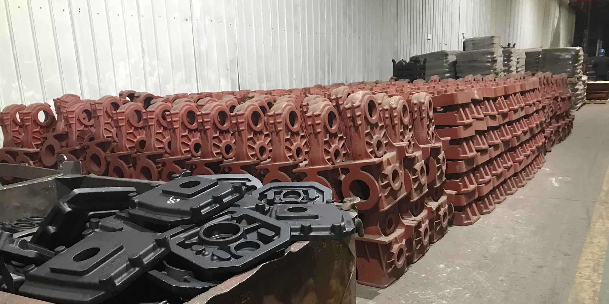
As the construction industry evolves, building structures are becoming increasingly large-span and architecturally diverse. Steel castings offer significant design freedom, allowing for shapes tailored to structural stress conditions and pouring processes. Furthermore, because steel casting nodes are integrally cast, they effectively reduce stress concentration and improve mechanical performance. Consequently, steel castings have become increasingly prevalent in stadiums, railway stations, large plazas, and other buildings. However, civil engineering codes typically treat cast steel as an ideal, continuous, homogeneous material when calculating bearing capacity. In reality, due to limitations in casting technology and the influence of environmental factors, various casting defects inevitably arise during production. These defects can, to a certain extent, affect the mechanical properties of steel castings and even the overall structure, potentially threatening structural safety. Despite this, the engineering community has not paid sufficient attention to defects, and scholarly research on their impact remains insufficient. Usually, the existence of defects is either ignored in engineering practice or accounted for by increasing the safety factor, leading to inaccurate safety assessments of steel casting nodes and increased engineering costs.
To study the impact of casting defects on the mechanical properties of steel castings, this thesis focuses on two aspects: the influence of macroscopic casting defects and that of microscopic defects. The primary work is structured as follows.
1. Macroscopic Casting Defect Statistical Analysis and Prediction
1.1 Slicing Test of Steel Casting
I conducted a slicing test on a typical four-branch steel casting node to obtain precise information on internal macroscopic casting defects. The steel casting node measured 860 mm × 750 mm, weighing 0.608 tons, with a 50 mm thick annular stiffener at the mid-section of the main pipe. The test procedure involved both band sawing and water jet cutting. The band saw was an H-7056 large-type machine, while the water jet cutter was a DWJ1525FB three-axis cantilever machine with a cutting accuracy of ±0.10 mm and a maximum water pressure of 350 MPa.
The four-branch node was first cut parallel to the main pipe’s cross-section into 15 large rings at 50–80 mm intervals, yielding 14 large main-pipe cross-sections labeled A through N. Subsequently, the branch pipes were cut into 11 blocks, producing 10 branch sections labeled a through j. The main pipe rings were further divided: the four end rings were each cut into 6 small blocks, while the eleven mid-section rings—containing stiffeners and intersecting branch pipes—required more complex cutting. The N-6 block (at the main-branch connection) was further divided into four sub-blocks (N-6 to N-9). In total, the slicing test produced 121 blocks and 144 sections.
1.2 Statistical Analysis of Casting Defects
I classified defects according to Table 1 and counted the number, size, and location of each defect type on all 144 sections.
| Defect Name | Characteristics | Causes |
|---|---|---|
| Porosity | Smooth inner walls | Intrusive, precipitated, and reaction gases |
| Inclusion | Metallic or non-metallic inclusions | Indigenous or exogenous, complex reasons |
| Hot cracking | Penetrating or non-penetrating tortuous cracks | Large thickness differences, insufficient fillet radii, restrained contraction |
| Cold cracking | Straight, elongated cracks | Large wall thickness differences, excessive temperature gradients |
| Shrinkage cavity | Scattered or concentrated macro-holes with dendrites and inclusions | Poor feeding at final solidification locations, prolonged solidification |
| Shrinkage porosity | Dispersed interdendritic holes, often below shrinkage cavities | Fine shrinkage porosity is unavoidable |
| Delamination | Long banded distribution | Complex origins |
| Unfused chaplet | Residual chaplets or internal chills not fully melted | Incomplete fusion during pouring |
Among the 337 macroscopic defects found on 74 defective sections, the distribution was: 142 in the outer layer, 114 in the middle layer, and 73 in the inner layer. The outer layer contained the most defects, while the inner layer had the fewest. Notably, among the 64 porosity defects, 78.13% resided in the outer layer, indicating a strong correlation between gas porosity and position—gases were more likely to remain near the exterior during pouring. Conversely, among 176 shrinkage-related defects, 104 (59.09%) were found in the middle layer because the middle layer cools and solidifies more slowly, leading to feeding deficiencies. For the 84 inclusion defects, 51.19% were in the outer layer, 40.48% in the inner layer, and only 8.33% in the middle layer.
In terms of defect types among all 337 defects, shrinkage cavities and porosity accounted for 52.23%, inclusions for 24.93%, and gas porosity for 18.99%. Together, the hole-type defects represented 71.22% of the total, confirming that shrinkage-related and gas-related defects were the dominant macroscopic defect types in this steel casting.
Defect size statistics revealed a clear inverse relationship between size and frequency. Smaller defects dominated: 265 defects (81.4%) were smaller than 6 mm, while only a handful exceeded 30 mm. The distribution histogram showed that the majority of macroscopic defects in steel castings are of small size, which is an important consideration for quality assessment and structural integrity evaluation.
1.3 Maximum Defect Size Prediction Model
To provide a practical tool for engineering quality assessment and for subsequent mechanical analyses, I developed a predictive model for the maximum defect size on a given section based on the counts of various defect types. I employed support vector regression (SVR), a machine learning method well-suited for small-sample problems.
Given a training dataset {(x₁,y₁),…,(xₙ,yₙ)} with input vector x and output y, the SVR model seeks a function that deviates from the actual targets by no more than ε while being as flat as possible. For nonlinear problems, a kernel function maps the input into a higher-dimensional feature space. I used the Gaussian (radial basis function) kernel:
$$ k(\mathbf{x}_i, \mathbf{x}) = \exp\left(-\frac{\|\mathbf{x}_i – \mathbf{x}\|^2}{\sigma^2}\right) $$
where σ is the kernel hyperparameter optimized by grid search.
I used data from 72 sections with inclusions, shrinkage cavities, gas porosity, and shrinkage porosity counts as the four input features and the maximum defect size as the output. Among these, 67 sections formed the training set and 5 formed the validation set. Table 2 lists the prediction results.
| Actual max defect size (mm) | Predicted max defect size (mm) | Relative error (%) |
|---|---|---|
| 2.5 | 2.2 | 12.0 |
| 1.8 | 2.1 | 16.7 |
| 13.5 | 12.9 | 4.4 |
| 3.2 | 3.0 | 6.3 |
| 2.9 | 3.3 | 13.8 |
I computed the mean squared error (MSE) of the model:
$$ \text{MSE} = \frac{1}{N} \sum_{t=1}^{N} (\text{observed}_t – \text{predicted}_t)^2 $$
An MSE value of 14.8% (below the 20% threshold) indicated that the prediction model performed well and could be used as a reference for engineering-quality assessment of geometrically similar steel casting components. This model also provides a rational basis for determining defect dimensions in finite element analysis of steel casting mechanical behavior.
2. Influence of Macroscopic Casting Defects on Mechanical Properties of Steel Casting Nodes
2.1 Finite Element Modeling
To study the influence of macroscopic casting defects on the mechanical properties of steel castings, I analyzed a typical K-type G20Mn5N steel casting node using ABAQUS with a linear hardening elastoplastic model. The material properties, as determined from uniaxial tensile tests, are listed in Table 3.
| Property | Elastic modulus (GPa) | Poisson’s ratio | Initial yield strength (MPa) | Initial yield strain | Plastic modulus (GPa) | Ultimate strength (MPa) | Ultimate strain |
|---|---|---|---|---|---|---|---|
| Value | 230 | 0.3 | 320 | 0.00139 | 1.35 | 586 | 0.205 |
The linear hardening elastoplastic stress–strain model was expressed as:
$$ \sigma = \begin{cases} E\varepsilon, & \sigma \leq \sigma_y \\ \sigma_y + H(\varepsilon – \varepsilon_y), & \sigma > \sigma_y \end{cases} $$
Three steel casting node models were created using SolidWorks and imported into ABAQUS: Model 1 – no macroscopic casting defects (the pristine node); Model 2 – containing a single macroscopic defect (a spherical gas pore of radius 3 mm); Model 3 – containing multiple macroscopic casting defects (one gas pore and two inclusion-type defects). Based on the statistics from the slicing test, the highest probability of defect occurrence was at the intersection between the main and branch pipes. The defect sizes were consistent with the prediction model: a single gas pore corresponds to approximately 6 mm diameter, and a single inclusion corresponds to approximately 13 mm. All defects were placed in the outer layer.
Both main-pipe ends were constrained as fixed. Concentrated loads F1 and F2 of equal magnitude were applied along the axes of the two branch pipes. I used C3D10 tetrahedral elements with a global mesh size of 15 mm and a local mesh size of 2 mm around the defects.
2.2 Strength Analysis
With F1 = F2 = 850 kN, the computed Mises stress distributions for all three models are shown. The overall stress distributions were nearly identical across the three models. The maximum Mises stress values were 419.2 MPa, 424.4 MPa, and 430.3 MPa for Models 1, 2, and 3, respectively, showing a slight increase in stress with an increasing number of defects.
However, the local effects were more significant. At the location of the macroscopic defect (“point M2”), the stress was 320.32 MPa, whereas in the defect-free model, the stress at the corresponding location (“point M1”) was only 250.57 MPa. The stress concentration factor was calculated as:
$$ \text{SCF} = \frac{\sigma_{\text{defect}}}{\sigma_{\text{no defect}}} = \frac{320.32}{250.57} = 1.278 $$
For the multi-defect model at “point M3”, the stress was 322.98 MPa, giving SCF = 1.289. This confirms that the presence of macroscopic casting defects significantly elevates local stresses, causing early yielding of the surrounding material even when the overall node remains elastic.
2.3 Stiffness and Ultimate Load Capacity Analysis
The displacement distributions for the three models were identical. The maximum displacement values were 0.7601 mm, 0.7613 mm, and 0.7618 mm, respectively. The difference was less than 0.01 mm, indicating that a small number of macroscopic defects had a negligible influence on the overall stiffness of the steel casting. However, as defect numbers increase, the stiffness degradation would become more pronounced.
I also investigated the ultimate bearing capacity by progressively increasing the loads and recording the load–displacement relationship at the branch pipe end. Figure 11 shows the load–displacement curves, and Figure 12 shows the corresponding stiffness–load curves. The initial stiffness values for Models 1, 2, and 3 were 1.138×10⁹ N/m, 1.127×10⁹ N/m, and 1.126×10⁹ N/m, respectively. According to the JGJ/T 395-2017 specification, the ultimate load corresponds to a stiffness reduction to 10% of the initial stiffness. The corresponding ultimate capacities were 1589 kN, 1582 kN, and 1578.5 kN. Thus, the presence of macroscopic casting defects reduces the ultimate bearing capacity of steel castings, although the reduction was relatively small for a single defect. The trend implies that with more defects, the ultimate load capacity will continue to decrease.
2.4 Fatigue Analysis of Steel Casting Nodes
Macroscopic defects significantly influence fatigue performance. The stress range Δσ is given by:
$$ \Delta\sigma = \frac{\sigma_{\max} – \sigma_{\min}}{2} $$
Using the G20Mn5N S-N curve at a 99% survival rate, I applied a cyclic load between −500 kN and +1000 kN (ΔF = 1500 kN) and extracted the stresses at the critical locations. The results are summarized in Table 4.
| Position | Peak value (MPa) | Valley value (MPa) | Stress amplitude (MPa) | Fatigue life (cycles) | Life reduction vs. Model 1 |
|---|---|---|---|---|---|
| Model 1 point M1 | 296.713 | 142.919 | 219.82 | 247,685 | — |
| Model 2 point M2 | 345.505 | 201.018 | 273.26 | 20,417 | 91.7% |
| Model 3 point M3 | 347.881 | 203.816 | 275.85 | 18,268 | 92.6% |
The presence of a single macroscopic defect reduced the fatigue life of the steel casting node by more than 90%, which is a dramatic and dangerous effect. This finding highlights that macroscopic casting defects are critical for the safety and durability of steel castings under cyclic loading.
3. Lemaitre Damage Model for Steel Castings
3.1 Fundamental Theory of the Lemaitre Damage Model
To investigate the influence of microscopic defects on the mechanical performance of steel castings, I adopted the Lemaitre damage model within the framework of continuum damage mechanics. The theory is built on four fundamental concepts: the damage variable, the isotropic damage assumption, effective stress, and the strain equivalence hypothesis.
The damage variable D is defined as the ratio of the damaged area to the total area of a representative volume element:
$$ D = \frac{A_D}{A} = \frac{A – \tilde{A}}{A} $$
where A is the total cross-sectional area, and Ā is the effective load-bearing area. When D = 0, the material is undamaged; when D = D_C, complete fracture occurs.
The effective stress tensor is given by:
$$ \tilde{\sigma}_{ij} = \frac{\sigma_{ij}}{1 – D} $$
According to the strain equivalence hypothesis, the constitutive relationship of the damaged material can be expressed using the same form as the undamaged material, but with the effective stress replacing the nominal stress:
$$ \varepsilon_{ij}^e = \frac{1 + \nu}{E} \frac{\sigma_{ij}}{1-D} – \frac{\nu}{E} \frac{\sigma_{kk}}{1-D}\delta_{ij} $$
Based on thermodynamic principles, the damage energy release rate Y is derived from the elastic strain energy. For isotropic materials, it can be expressed as:
$$ Y = \frac{\tilde{\sigma}_{eq}^2}{2E(1-D)^2} R_\nu $$
where the stress triaxiality function R_ν is defined as:
$$ R_\nu = \frac{2}{3}(1+\nu) + 3(1-2\nu)\left(\frac{\sigma_m}{\sigma_{eq}}\right)^2 $$
Here, σ_eq is the Mises equivalent stress and σ_m is the hydrostatic stress. The damage evolution law is:
$$ \dot{D} = \left(\frac{Y}{S_0}\right)^{\alpha_0} \frac{\dot{\varepsilon}_{pl}}{(1-D)} $$
where S₀ and α are material damage parameters. For ductile metals, α is typically set to zero. Combining all equations yields the complete Lemaitre damage constitutive model:
$$ \begin{cases} \boldsymbol{\sigma} = (1-D)\mathbf{D}^e : (\boldsymbol{\varepsilon} – \boldsymbol{\varepsilon}_p) \\ \dot{\boldsymbol{\varepsilon}}_p = \dot{\lambda} \frac{\partial F}{\partial \boldsymbol{\sigma}} \\ \dot{D} = \frac{Y}{S_0(1-D)} \dot{\varepsilon}_p \end{cases} $$
3.2 Numerical Integration Algorithm for Steel Casting Simulation
I implemented a return mapping algorithm based on the backward Euler method to solve the Lemaitre elastoplastic damage constitutive equations. The process begins with an elastic predictor step. Assuming all strain increments are elastic, the trial stress is:
$$ \boldsymbol{\sigma}_{tr} = \boldsymbol{\sigma}_n + (1-D_n)\mathbf{D}^e : \Delta\boldsymbol{\varepsilon} $$
where σₙ and Dₙ are the stress and damage at the previous increment. The trial yield function is then evaluated:
$$ f_{tr} = \frac{3}{2} \tilde{\boldsymbol{\eta}}_{tr} : \tilde{\boldsymbol{\eta}}_{tr} – H – \sigma_{y,0} $$
with the effective trial deviatoric stress given by:
$$ \tilde{\boldsymbol{\eta}}_{tr} = \frac{\mathbf{S}_{tr}}{1-D_n} $$
If f_tr ≤ 0, the step is purely elastic with no damage evolution, and the stress, plastic strain, and damage state variables are updated trivially. If f_tr > 0, plastic deformation and damage evolution occur. The plastic consistency parameter is:
$$ \hat{\gamma} = \frac{f_{tr}}{2\mu + \frac{3}{2}H} $$
The updated stress tensor is:
$$ \boldsymbol{\sigma}_{n+1} = \boldsymbol{\sigma}_{tr} – 2\mu\hat{\gamma}(1-D_{n+1})\tilde{\mathbf{N}}_{n+1} $$
where Ñ is the unit flow direction at the updated state. The accumulated plastic strain update is:
$$ \varepsilon_{pl,n+1} = \varepsilon_{pl,n} + \sqrt{\frac{2}{3}}\hat{\gamma} $$
Finally, the damage variable is updated using:
$$ D_{n+1} = D_n + \frac{\sigma_{eq,n+1}^2 R_{\nu,n+1} \Delta\varepsilon_p}{2E S_0 (1-D_n)^2} $$
This numerical integration scheme is implemented in a UMAT user subroutine for ABAQUS. The computational flow is illustrated schematically as follows: (1) read the state variables at step n; (2) compute the external and internal force vectors; (3) check convergence; (4) solve for the displacement and strain increments; (5) compute the trial stress and trial yield function; (6) if yielding occurs, compute the plastic multiplier and the updated flow direction; (7) update the stress, plastic strain, and damage; (8) store the state variables.
3.3 Parameter Determination for the Steel Casting Material
To determine the Lemaitre damage parameters, I utilized notched-bar tensile tests and X-ray computed tomography (CT) scanning. Three types of G20Mn5N steel casting notched specimens with notch radii of 2 mm, 6 mm, and 10 mm (designated as R2, R6, and R10) were tested. For each type, four specimens were prepared. Three specimens were subjected to monotonic tensile loading to obtain the average load–displacement curve. The fourth specimen was loaded to eight predetermined unloading points sequentially, and at each point, an X-ray CT scan was performed to measure the internal microdefect volume fraction. The CT system was a Y.CT Precision System industrial tomograph.
The damage variable D was related to the measured volume fraction f through the following geometric conversion. Assuming spherical defects, the radius ratio is:
$$ \delta = \frac{r}{R} = \left(\frac{3f}{4\pi}\right)^{1/3} $$
Then the area fraction (which is the damage variable) is:
$$ D = \frac{1}{2} – \frac{1}{2}\delta^2 – \frac{1}{4}\ln\left(\frac{1-\delta}{1+\delta}\right)(1-\delta^2) $$
I converted the measured volume fractions to damage variables for all three specimen types at each loading stage. The initial damage variable D₀, corresponding to the undamaged state, was computed as the average of the initial damage values of the R2, R6, and R10 specimens: D₀ = 0.00181. Similarly, the critical damage variable D_C was determined as the average damage value at the last scan before fracture: D_C = 0.0308.
The material damage parameter S₀ was determined using a semi-empirical equation that relates it to the critical damage, the ultimate strength, and the elongation at fracture:
$$ S_0 = \frac{E \left( \frac{\sigma_u}{1.65} \right)^{1+n’} }{2 (1+n’)} \left( \frac{1}{\ln(\varepsilon_f / 0.59)} \right) $$
where E = 230 GPa, σ_u = 586 MPa, n’ = 0.15, ε_f = 0.59, and c = −0.58. Substituting these values yielded S₀ = 18.19 MPa. For the damage exponent α₀, I set α = 1, which is the common value for ductile metallic materials. The complete set of Lemaitre damage parameters for G20Mn5N steel casting is listed in Table 5.
| E (GPa) | ν | σ_y0 (MPa) | ε_y0 | H (GPa) | σ_u (MPa) | D₀ | S₀ (MPa) | α | D_C |
|---|---|---|---|---|---|---|---|---|---|
| 230 | 0.3 | 320 | 0.00139 | 1.35 | 586 | 0.00181 | 18.19 | 1 | 0.0308 |
4. Effects of Microscopic Defects on Mechanical Properties of Steel Casting Nodes
4.1 UMAT Subroutine Development and Validation
I developed an ABAQUS UMAT user subroutine implementing the Lemaitre damage model with the return mapping algorithm described in Section 3.2. To validate the subroutine, I created finite element models of the notched-bar specimens with the same geometry as those used in the CT experiments. The models were meshed with C3D8R elements, with a mesh size of 2 mm globally and 0.5 mm near the notch to resolve the high damage gradients.
The computed damage variable–equivalent plastic strain curves were compared with both the experimental CT measurement data and the GTN damage model results from a previous study on the same G20Mn5N steel casting material. The GTN (Gurson–Tvergaard–Needleman) model is a micromechanics-based damage model that explicitly accounts for void nucleation, growth, and coalescence. The comparison is shown for the R2, R6, and R10 specimens. Both the Lemaitre and GTN models captured the experimental trend reasonably well: damage accumulates slowly in the early stages of plastic deformation and accelerates as the equivalent plastic strain increases. The GTN model provided a slightly better fit because it was specifically calibrated for void evolution. However, the Lemaitre model performed satisfactorily with an acceptable accuracy for the purpose of assessing the influence on mechanical properties. This confirmed the correctness of the determined material parameters and the reliability of the UMAT subroutine.
I further examined the damage evolution in specimen R6 by monitoring the damage variable distribution at various load steps. At the initial state, the damage was uniformly distributed at the initial value D₀ = 0.00181. As the displacement load increased, damage accumulated progressively around the notch. The damage values increased from 0.00181 at the initial state to values exceeding the critical damage D_C in the most stressed zones. The region of active damage evolution expanded outward from the notch, indicating that microscopic defects initiated, grew, and coalesced under continued loading, which would eventually lead to macroscopic crack formation.
4.2 Finite Element Analysis of a K-type Steel Casting Node with Microscopic Defects
To investigate the impact of microscopic defects on realistic steel casting components, I performed finite element analyses on the same three K-type G20Mn5N steel casting node models (Model 1: no macroscopic defects; Model 2: one macro-defect; Model 3: multiple macro-defects), this time using the Lemaitre damage model. The loading and boundary conditions were identical to those in Section 2.1.
Under a static load of F1 = F2 = 850 kN, the Mises stress contour plots showed that the overall stress distributions were nearly identical among the three models and similar to those obtained with the linear hardening elastoplastic model. The maximum Mises stresses were 410.9 MPa, 423.5 MPa, and 429.4 MPa for Models 1, 2, and 3, respectively. Comparing these with the linear hardening model results (419.2 MPa, 424.4 MPa, and 430.3 MPa), the difference was less than 2%. This indicates that, under static loading, the damage evolution of microscopic defects has a negligible influence on the overall strength of the steel casting node.
However, the local stress concentration factors at the macroscopic defect locations were affected by the microscopic damage evolution. For Model 2, the stress at “point M2” was 320.22 MPa, and for Model 3, the stress at “point M3” was 323.53 MPa. The stress concentration factors were:
$$ \text{SCF}_{\text{Lemaitre, Model 2}} = \frac{320.22}{246.59} = 1.299 $$
$$ \text{SCF}_{\text{Lemaitre, Model 3}} = \frac{323.53}{246.59} = 1.312 $$
These are slightly higher than the values (1.278 and 1.289) obtained from the linear hardening model without considering microscopic damage. This confirms that the damage evolution of microscopic defects increases the stress concentration around macroscopic defects. In other words, neglecting microscopic defects leads to an underestimation of the true local stress intensity, which is a safety concern for structural design.
4.3 Stiffness and Ultimate Capacity
The maximum displacement values from the Lemaitre damage model for Models 1, 2, and 3 were 0.7617 mm, 0.7627 mm, and 0.7632 mm, respectively. Compared with the linear hardening results (0.7601 mm, 0.7613 mm, 0.7618 mm), the additional displacement due to microdefect damage evolution was less than 0.01 mm. Thus, microscopic defects have a negligible influence on the stiffness of steel castings under static loading.
For the ultimate bearing capacity, I analyzed the defect-free steel casting node (Model 1) under both the linear hardening model and the Lemaitre damage model. The load–displacement curves were nearly coincident. The initial stiffness values were 1.138×10⁹ N/m (linear hardening) and 1.125×10⁹ N/m (Lemaitre damage). The corresponding ultimate loads were 1589 kN and 1583.5 kN. The ultimate load decreased by approximately 0.3%, indicating a small but non-negligible effect of microscopic damage evolution on the ultimate capacity of steel casting nodes.
4.4 Damage Evolution Analysis for Steel Casting Nodes
Under a static load of 1000 kN, the damage fields for Model 1 (no macroscopic defects) and Model 2 (one macroscopic defect) were compared. Both models exhibited damage evolution at the fixed support regions and at the main–branch intersections. The presence of a macroscopic defect increased the maximum damage variable from 1.845×10⁻³ to 1.854×10⁻³ and significantly expanded the region over which damage evolved at the main-branch intersection. This finding indicates that the coexistence of macroscopic and microscopic defects is more harmful than either type alone, confirming that macro-defects magnify the damage evolution of microscopic defects.
Under cyclic loading (−500 kN to +1000 kN), the damage variable in the steel casting node increased monotonically with the number of cycles, even though stress and displacement cycled. The damage evolution region expanded outward continuously. This irreversible nature of the damage evolution process is a fundamental characteristic of continuum damage mechanics and has important implications for the fatigue life prediction of steel castings. Once damage accumulates, it cannot be reversed, and the material properties are permanently degraded.
5. Reliability Analysis of Steel Castings Considering Random Microscopic Defects
5.1 Statistical Distribution of Initial Defect Volume Fraction
The initial microdefect volume fraction in a steel casting is inherently random due to variations in alloy composition, casting process parameters, casting geometry, and environmental conditions. To characterize this randomness, I analyzed the initial defect volume fractions measured from 9 notched-bar specimens in the X-ray CT experiments: 0.00156, 0.00176, 0.00184, 0.00276, 0.003, 0.00307, 0.00327, 0.00373, and 0.00484.
Given the small sample size (n = 9), I applied the Shapiro–Wilk test, which is specifically designed for normality testing of small samples (n ≤ 50). The test statistic W is computed as:
$$ W = \frac{\left( \sum_{i=1}^{m} a_{in}(x_{n-i+1} – x_i) \right)^2}{\sum_{i=1}^{n}(x_i – \bar{x})^2} $$
where a_in are tabulated coefficients and m = n/2 for even n or (n+1)/2 for odd n. I computed W = 0.938 with n = 9. Using a significance level of α = 0.05, the critical value from the Shapiro–Wilk table for n = 9 is W(0.05, 9) = 0.829. Since 0.938 > 0.829, the null hypothesis of normality was not rejected. Thus, the initial defect volume fraction was considered to follow a normal distribution.
I calculated the sample mean and standard deviation as:
$$ \mu_f = 0.00287, \quad \sigma_f = 0.001052, \quad \sigma_f^2 = 0.000001107 $$
The probability density function of the initial defect volume fraction is:
$$ f(f) = \frac{1}{0.001052\sqrt{2\pi}} \exp\left[-\frac{(f – 0.00287)^2}{2(0.001052)^2}\right] $$
5.2 Material Property Degradation Due to Microscopic Defects
Based on the experimental relationships proposed by Hardin and Beckermann, the elastic modulus E and Poisson’s ratio ν of a steel casting with a defect volume fraction f can be expressed as:
$$ E(f) = E_0 \left(1 – \frac{f}{0.5}\right)^{0.5} $$
$$ \nu(f) = \nu_0 + (\nu_\infty – \nu_0)\frac{f}{f_\infty} $$
where E₀ = 230 GPa, ν₀ = 0.3, ν∞ = 0.14, and f∞ = 0.045. These relationships convert the random defect volume fraction into random material properties, allowing the uncertainty to be propagated through structural analyses.
5.3 Reliability Analysis Methods
Structural reliability is defined as the probability that a structure will perform its intended functions within a specified period under specified conditions. The limit state is described by a performance function:
$$ Z = g(\mathbf{X}) = g(X_1, X_2, \ldots, X_n) $$
where X represents the vector of basic random variables. When Z > 0, the structure is safe; when Z < 0, failure occurs. The failure probability is:
$$ P_f = P(Z < 0) = \int_{-\infty}^{0} f_Z(z) dz $$
where f_Z(z) is the probability density function of Z. When Z follows a normal distribution, the reliability index β is defined as:
$$ \beta = \frac{\mu_Z}{\sigma_Z} $$
and the failure probability is related to β through the standard normal cumulative distribution function:
$$ P_f = \Phi(-\beta) = 1 – \Phi(\beta) $$
I used two methods to evaluate the reliability of a steel casting plate: the first-order second-moment (FOSM) method with the Taylor expansion stochastic finite element method, and the Monte Carlo stochastic finite element method.
5.3.1 First-Order Second-Moment Method
The FOSM method expands the performance function in a first-order Taylor series around the mean values of the random variables:
$$ Z \approx g(\boldsymbol{\mu}_X) + \sum_{i=1}^{n} \frac{\partial g}{\partial X_i}\bigg|_{\boldsymbol{\mu}_X} (X_i – \mu_{X_i}) $$
The mean and variance of Z are then:
$$ \mu_Z = g(\boldsymbol{\mu}_X) $$
$$ \sigma_Z^2 = \sum_{i=1}^{n} \left( \frac{\partial g}{\partial X_i}\bigg|_{\boldsymbol{\mu}_X} \right)^2 \sigma_{X_i}^2 $$
In the finite element context, the displacement response is a function of the random material properties. I used the Taylor expansion stochastic finite element method, which requires the derivative of the displacement with respect to the random variable. To compute this derivative efficiently and accurately, I employed the complex variable differentiation method. For a function f(x), the derivative is:
$$ \frac{df}{dx} = \frac{\text{Im}[f(x + ih)]}{h} $$
where h is a small perturbation (taken as 10⁻¹⁰), and Im denotes the imaginary part. This method avoids the tedious analytical differentiation of matrix functions and provides highly accurate results.
I analyzed a 600 mm × 600 mm × 10 mm steel casting plate with one-quarter symmetry modeled in MATLAB. A uniform load of 1600 kN was applied at the top edge, with symmetric boundary conditions on the two symmetry planes. The free-end corner point A had the maximum displacement, making it the critical location. The displacement was computed as a function of the random defect volume fraction.
The mean displacement was calculated as 0.282294 mm, and the variance was 2.2304×10⁻¹². Assuming the ultimate displacement limit was 0.286 mm, the performance function is:
$$ Z = 0.286 – u(f) $$
The reliability index was:
$$ \beta = \frac{0.286 – 0.282294}{\sqrt{2.2304 \times 10^{-12} \times \left(\frac{\partial u}{\partial f}\right)^2 \sigma_f^2}} = 2.3261 $$
The failure probability was:
$$ P_f = \Phi(-\beta) = \Phi(-2.3261) = 0.01048 $$
Since β = 2.3261 < 3.0902, the failure probability estimate is insensitive to the distribution type of Z, and the normal approximation is acceptable for engineering purposes.
5.3.2 Monte Carlo Method
The Monte Carlo method uses repeated random sampling to estimate the probability of failure. For each sample, the steel casting plate finite element analysis was solved, and the displacement at point A was compared with the limit value. The failure probability is estimated as:
$$ \hat{P}_f = \frac{1}{N} \sum_{i=1}^{N} I[g(\mathbf{X}_i) < 0] $$
where I[·] is an indicator function equal to 1 when the limit state is violated and 0 otherwise. I generated N random samples of the defect volume fraction from the normal distribution N(0.00287, 0.000001107) and computed the corresponding displacement for each sample.
I analyzed the convergence behavior of the displacement mean as a function of the sample size. With N = 5000, the mean fluctuated noticeably around 0.0002823 m. With N = 50,000, the mean converged to a stable value of 0.00028230 m. The variance computed from the Monte Carlo simulation was 2.2610×10⁻¹². The frequency distribution histogram of the displacement showed that the most likely displacement range was between 0.281 mm and 0.283 mm.
With N = 50,000 samples and the displacement limit of 0.286 mm, I found that 49,492 samples satisfied the limit state. The failure probability was estimated as:
$$ \hat{P}_f = \frac{50,000 – 49,492}{50,000} = \frac{508}{50,000} = 0.01016 $$
To check the acceptability of this estimate, I computed the coefficient of variation:
$$ \text{COV}(\hat{P}_f) = \sqrt{\frac{1 – \hat{P}_f}{N \hat{P}_f}} = \sqrt{\frac{1 – 0.01016}{50,000 \times 0.01016}} \approx 0.044 $$
Since COV = 0.044 ≤ 0.05, the Monte Carlo estimate was deemed acceptable.
5.4 Comparison of Methods and Results
Table 6 compares the results obtained from the two reliability analysis methods for the steel casting plate.
| Quantity | FOSM | Monte Carlo | Relative error |
|---|---|---|---|
| Mean displacement (m) | 0.000282294 | 0.000282300 | 3.54×10⁻⁵ |
| Variance | 2.2304×10⁻¹² | 2.2610×10⁻¹² | 0.014 |
| Failure probability | 0.01048 | 0.01016 | 0.031 |
The relative errors between the two methods were extremely small—approximately 0.0035% for the mean displacement, 1.4% for the variance, and 3.1% for the failure probability—confirming the consistency and accuracy of both approaches. Both methods yielded a failure probability of approximately 1% for the steel casting plate when the displacement limit was set to 0.286 mm.
Notably, when the randomness of microscopic defects was neglected, the deterministic finite element analysis gave a displacement of 0.282 mm, which is less than the limit of 0.286 mm. This would suggest that the structure is completely safe. However, both reliability analyses revealed that the steel casting plate still has approximately a 1% chance of failure due to the inherent randomness of microdefects. This demonstrates the importance of accounting for defect randomness in the design of high-safety-class steel castings.
The comparison of the two methods reveals their respective advantages and limitations:
| Aspect | FOSM | Monte Carlo |
|---|---|---|
| Computational cost | Low (a few finite element solves) | High (many repeated finite element solves) |
| Accuracy | Moderate (first-order approximation) | High (sufficient sampling) |
| Applicability | Limited (small variability, low nonlinearity) | Wide (any distribution, any complexity) |
| Information obtained | Only first two moments | Full distribution of response |
The FOSM method is particularly efficient for problems with small variability (coefficient of variation < 0.3) and mild nonlinearity. The use of the complex variable differentiation method effectively streamlines the computation of the derivatives required by the Taylor expansion stochastic finite element method. However, the FOSM method relies on the assumption that the performance function is approximately linear and that Z follows a normal distribution, which may not hold for highly nonlinear or heavily skewed distributions.
The Monte Carlo method is straightforward to implement, can handle any distribution type and any degree of nonlinearity, and provides complete distribution information about the response. Its main drawback is the computational cost, as a large number of simulations are required to obtain accurate estimates of small failure probabilities. Nevertheless, with modern computational capabilities and variance-reduction techniques, the Monte Carlo method is increasingly practical and widely used for complex steel casting structures.
6. Conclusions
In this thesis, I systematically investigated the effects of casting defects on the mechanical properties of steel castings through a combination of experimental, numerical, and reliability analyses. The main findings and conclusions are as follows:
1) The slicing test of a typical four-branch steel casting node revealed the statistical distribution characteristics of macroscopic casting defects. Hole-type defects (shrinkage cavities, shrinkage porosity, and gas porosity) dominated, accounting for over 70% of all defects. The defect type was strongly correlated with the position: porosity defects occurred predominantly in the outer layer, shrinkage defects in the middle layer, and inclusions in the inner and outer layers. The highest defect density was found at the intersection between the main and branch pipes. This comprehensive dataset provides a solid foundation for understanding the defect characteristics of steel castings.
2) Using a support vector regression model with the Gaussian kernel, I established a prediction model that relates the counts of four defect types on a cross-section to the maximum defect size on that section. The model achieved a mean squared error of less than 15%, demonstrating good predictive accuracy. This model serves as a valuable reference for engineering quality assessment and provides a rational basis for defect size selection in the finite element analysis of steel castings.
3) The finite element analysis of a K-type G20Mn5N steel casting node, based on a linear hardening elastoplastic model, demonstrated that macroscopic casting defects do not change the overall stress distribution, but they significantly increase the local stress at the defect vicinity, producing stress concentrations with factors around 1.28–1.31. A small number of macro-defects had a negligible effect on the overall stress, stiffness, and ultimate bearing capacity. However, the fatigue life of the steel casting node was drastically reduced by over 90% in the presence of a single macro-defect, and by about 92.6% with multiple defects. These findings underline the critical importance of macro-defects for the fatigue durability of steel castings.
4) I determined the Lemaitre damage model parameters for G20Mn5N steel casting based on X-ray CT experiments on notched-bar specimens. The initial damage variable was D₀ = 0.00181, the critical damage was D_C = 0.0308, and the damage strength parameter was S₀ = 18.19 MPa. I implemented the model as an ABAQUS UMAT subroutine and validated it by comparing the simulated damage–strain curves with experimental data. The agreement was satisfactory, confirming the suitability of the Lemaitre damage model for describing the damage evolution behavior of steel castings under monotonic and cyclic loads.
5) The finite element analysis based on the Lemaitre damage model showed that microscopic defects have a minor influence on the overall stress (less than 2% difference), stiffness (less than 0.01 mm difference), and ultimate bearing capacity (approximately 0.3% reduction) of the steel casting node under static loading. However, when microscopic damage evolution was considered, the stress concentration factor around macroscopic defects increased, indicating that microscopic damage amplifies the adverse local effects of macroscopic defects. Conversely, the presence of macroscopic defects accelerates the damage evolution of microscopic defects. The damage accumulation was shown to be irreversible, which has important implications for the long-term integrity of steel castings.
6) The initial microdefect volume fraction in G20Mn5N steel castings follows a normal distribution N(0.00287, 0.000001107), as confirmed by the Shapiro–Wilk test. The randomness of this volume fraction was propagated through a reliability analysis of a steel casting plate using both the first-order second-moment (FOSM) method and the Monte Carlo method. The two methods yielded consistent results with relative errors below 3.1%. Both methods predicted a failure probability of approximately 1% for the plate under the specified load, despite the deterministic analysis indicating safety. This suggests that defect randomness must be considered in the reliability-based design of steel castings.
In conclusion, this thesis demonstrates that both macroscopic and microscopic casting defects have appreciable effects on the mechanical properties of steel castings. While the influence on overall elastic properties is relatively small, the local stress concentration and fatigue life reduction caused by macro-defects, as well as the damage amplification and randomness effects contributed by microscopic defects, cannot be ignored. The methods and findings presented in this thesis provide valuable insights for the design, quality assessment, and reliability-based optimization of steel castings in engineering applications.