
As a researcher in materials processing engineering, my work has focused on the development of robust numerical simulation techniques for predicting the microstructure and mechanical properties of steel casting components. Steel castings constitute approximately 15% of the total casting output in China and serve as critical components in machinery, transportation equipment, and heavy industrial applications. The service life and safety of mechanical parts are directly governed by the quality of the steel casting, which in turn is determined by its microstructure and performance characteristics. Therefore, the ability to precisely control and predict the microstructure distribution in steel casting is of paramount industrial importance.
Traditionally, the methods of casting and heat treatment have served as the principal means of controlling component microstructure. The former establishes the initial as-cast structure, while the latter refines this structure to achieve the final mechanical properties required for service. However, a significant gap exists in the numerical simulation community. Most established simulation tools treat these two essential processes independently. When solidification is simulated alone, the resulting as-cast structure and performance cannot directly define the final quality of the part, especially since heat treatment is often mandatory. Conversely, when the heat treatment process is simulated in isolation, the influence of the initial as-cast microstructure—which significantly affects phase transformation kinetics during heat treatment—is entirely neglected. This disconnect from physical reality undermines the accuracy and reliability of the simulation outcomes.
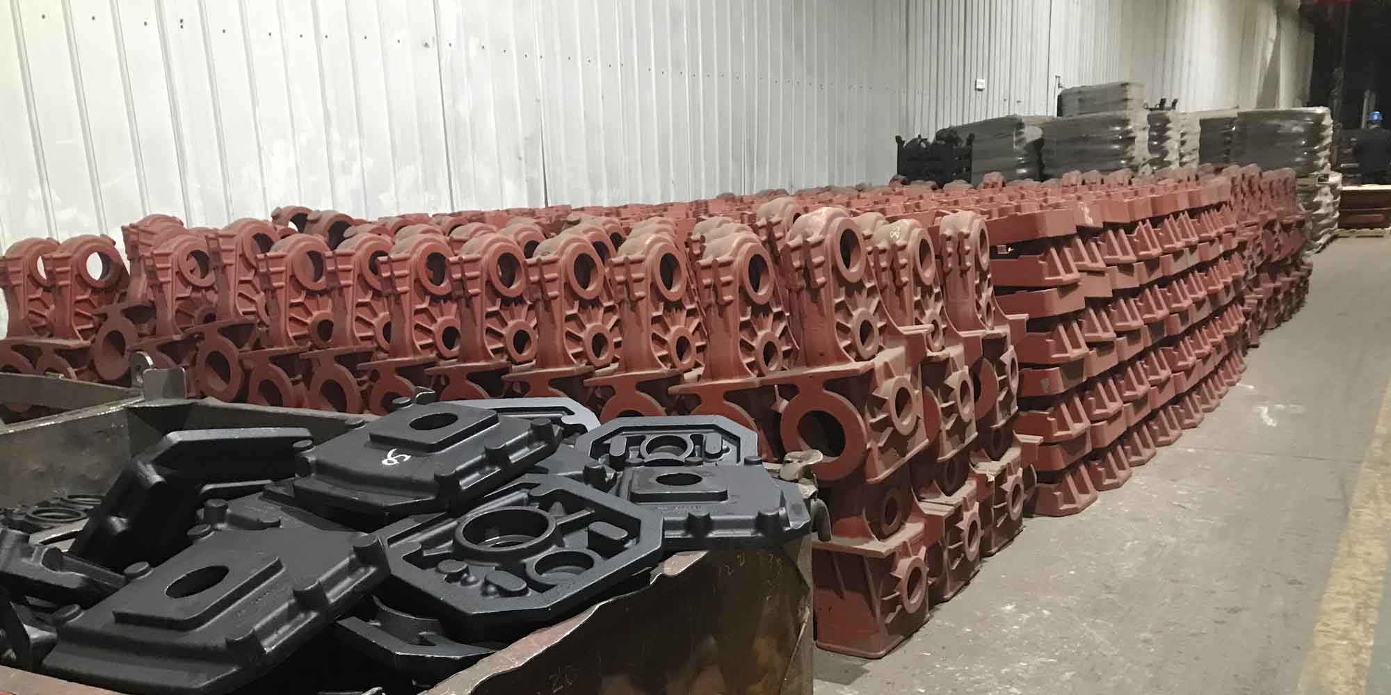
Motivated by this limitation, my research objective has been to bridge the gap between casting solidification and subsequent heat treatment through an integrated full-process simulation framework. By coupling these two stages using advanced mapping techniques, the simulation becomes a more faithful representation of the industrial reality. The methodology enables the accurate prediction of the microstructural evolution and the resulting mechanical property distribution in steel casting components. This integrated approach not only assists process engineers in visualizing and understanding the complete lifecycle of the component’s internal state but also provides a scientific basis for optimizing processing parameters to enhance overall quality. Throughout this thesis, I will refer to the subject material as steel casting, emphasizing its significance in the context of mechanical part fabrication. A key visualization of a typical steel casting component is provided below.
Numerical Simulation of the Solidification Process for Steel Casting
The accurate prediction of the solidification microstructure in steel casting is predicated on the precise calculation of the transient temperature field. The solidification process in a mold is characterized by complex heat transfer mechanisms, including conduction through the casting and mold, convection within the liquid metal, and radiation at exposed surfaces. For the purpose of this work, I assumed that the mold filling occurs instantaneously, allowing the initial temperature field to be considered uniform within both the metal and the mold. The governing equation for the three-dimensional heat conduction within the steel casting is based on the Fourier heat transfer law combined with the energy conservation principle.
The mathematical model for the temperature field during the solidification of a steel casting is expressed by the following partial differential equation:
$$ \rho C \frac{\partial T}{\partial t} = \lambda \left( \frac{\partial^2 T}{\partial x^2} + \frac{\partial^2 T}{\partial y^2} + \frac{\partial^2 T}{\partial z^2} \right) + Q $$
where \( \rho \) represents the density of the material, \( C \) is the specific heat capacity, \( T \) is the temperature at time \( t \), \( \lambda \) is the thermal conductivity, \( x, y, z \) represent the three-dimensional spatial coordinates, and \( Q \) is the internal heat source intensity, which accounts for the release of latent heat during phase transformation. The appropriate initial conditions are defined as \( T_{Cast} = T_{1} \) and \( T_{Mold} = T_{2} \) at time \( t = 0 \), where \( T_{1} \) is the initial metal temperature slightly below the pouring temperature and \( T_{2} \) is the initial mold temperature, typically at ambient conditions. The boundary conditions are classified into three types, with the third type—convective and radiative heat transfer at the casting surface—being the most relevant for the casting process.
To solve this continuous mathematical model, I employed the finite difference method (FDM) for discretization. As shown in my analysis of the heat balance for a control volume, the temperature of a node at the next time step is a linear combination of its current temperature and that of its six neighboring nodes. For a node \( i \) with a uniform grid spacing \( \Delta x \), the discretized form of the heat conduction equation can be derived as:
$$ T_i^{t+\Delta t} = T_i^t \left( 1 – \frac{a_i \Delta t}{\rho_i C_{pi} \Delta x} \right) + \frac{\Delta t}{\rho_i C_{pi} \Delta x} \sum_{j=1}^{6} \frac{T_j^t}{\frac{\Delta x}{2\lambda_i} + \frac{\Delta x}{2\lambda_j}} $$
where \( T_i^{t+\Delta t} \) is the temperature of node \( i \) at the new time step, and \( T_j^t \) refers to the temperatures of the adjacent nodes. The stability criterion for this explicit scheme requires that the coefficient of \( T_i^t \) remains non-negative, leading to the condition:
$$ \Delta t \leq \frac{\rho_i C_{pi} (\Delta x)^2}{a_i} $$
This ensures a convergent solution for the temperature field, forming the basis upon which the subsequent microstructure prediction is built.
In the simulation of the solidification of a steel casting, a critical aspect is the treatment of latent heat. I explored three primary methods for handling this phenomenon: the temperature recovery method, the equivalent specific heat method, and the enthalpy method. The temperature recovery method is particularly intuitive; it posits that the latent heat released during solidification compensates for the heat lost via conduction. The corresponding temperature rise \( \Delta T \) in a control volume can be expressed as:
$$ \Delta T = \frac{\Delta f_s \cdot L}{C_p} $$
where \( L \) is the latent heat of fusion and \( \Delta f_s \) represents the incremental increase in the solid fraction within a time step. This method is computationally efficient and is commonly integrated into casting simulation software for steel casting, such as the Huazhu CAE software utilized in my research.
Prediction Model for Solidification Microstructure and Performance in Steel Casting
The primary objective of simulating the solidification process in steel casting is to predict the final as-cast grain size, phase constitution, and mechanical properties. Due to the complex and often unknown parameters governing nucleation in industrial alloys, I adopted a pragmatic approach that couples macroscopic temperature field simulation with thermodynamic calculation databases.
For the prediction of grain size, I utilized the continuous nucleation model first proposed by Rappaz and Thevoz, which is based on a Gaussian distribution of nucleation sites. This model assumes that nucleation occurs on a distribution of potential nucleation sites, described by a continuous function \( dn/d(\Delta T) \). The grain density \( n(\Delta T) \) at a given undercooling \( \Delta T \) is obtained by integrating this distribution from zero up to the current undercooling:
$$ n(\Delta T) = \int_{0}^{\Delta T} \frac{dn}{d(\Delta T’)} d(\Delta T’) $$
The nucleation rate distribution is defined by the following Gaussian function:
$$ \frac{dn}{d(\Delta T)} = \frac{n_{max}}{\sqrt{2\pi} \Delta T_\sigma} \exp \left[ -\frac{1}{2} \left( \frac{\Delta T’ – \Delta T_N}{\Delta T_\sigma} \right)^2 \right] $$
In this equation, \( n_{max} \) is the maximum density of heterogeneous nucleation substrates, \( \Delta T_N \) represents the mean nucleation undercooling, and \( \Delta T_\sigma \) is the standard deviation of the undercooling. In the discrete numerical model, the increase in grain density \( \delta n \) during a time step \( \Delta t \) is calculated as the integral of this Gaussian function over the incremental increase in undercooling \( \delta(\Delta T) \).
Once the grain density \( n \) is known for a given control volume, the average grain size \( r \) can be derived. Assuming that the equiaxed grains are spherical and occupy the entire volume \( V \) of the cell, the volume per grain is \( 1/n \). The relationship between the grain radius and density is:
$$ r = \sqrt[3]{\frac{3}{4\pi n}} $$
This provides a direct link between the simulated thermal history and the final as-cast grain size distribution across the steel casting.
Accurately predicting the phase fractions (e.g., ferrite, pearlite, bainite, martensite) in a steel casting is a more intricate challenge due to the non-equilibrium cooling conditions present in different sections of the casting. To address this, I developed a methodology that capitalizes on the capabilities of the thermodynamic simulation software JMatPro. This software can calculate the phase fractions and mechanical properties (yield strength, tensile strength, and hardness) as functions of temperature for a specific steel grade at various continuous cooling rates. A snapshot of such data for steel grade ZG20Mn is shown in the accompanying figure, depicting transformations of austenite into ferrite, pearlite, bainite, and martensite.
My approach involved building a comprehensive database of phase content and mechanical properties for a wide range of steel casting grades, including ZG15, ZG20CrMo, ZG25, ZG30Mn, ZG40Mn, ZG45, ZG55, ZG65Mn, among more than 100 grades commonly used in steel casting production. The cooling rate range considered for the database is 0.03°C/s to 15°C/s, which effectively covers the cooling rates encountered in the majority of regions within a typical steel casting during solidification. To apply this data to a full three-dimensional casting, I developed algorithms for rapid data searching and grid assignment. The process is as follows:
1. The temperature field for the entire steel casting is computed using the finite difference method, providing a detailed thermal history for every node.
2. For each grid cell, the cooling rate \( V \) within the solid-liquid two-phase region is calculated by identifying the times \( t_1 \) and \( t_2 \) when the node’s temperature crosses the liquidus \( T_{liq} \) and solidus \( T_{sol} \), respectively.
3. Using this calculated cooling rate \( V \), a search is performed in the pre-established database to find the JMatPro data file that corresponds to the closest cooling rate.
4. The phase fraction and mechanical property values at various temperatures are then extracted from this file and assigned to the respective grid cell, constructing the complete property distribution map for the entire steel casting.
This method is computationally efficient and avoids the need for complex, physics-based phase transformation models, which are often difficult to calibrate for industrial alloys. This database-driven approach allows for the rapid and accurate prediction of the macro-scale distribution of microstructure in a steel casting.
Prediction Model for Heat Treatment Microstructure and Performance in Steel Casting
Heat treatment is the indispensable final stage in the production of high-quality steel casting components, as it refines the as-cast structure and enhances mechanical properties. My research extends the simulation methodology to the heat treatment process, thereby creating a full-cycle prediction capability. The foundation of this process is the mapping technology that transfers the final as-cast state of the steel casting from the solidification simulation grid to the heat treatment simulation grid. In this mapping, the casting geometry is retained, while the mold grids are replaced by the heating or cooling medium. Critical to this coupling is the transfer of the predicted as-cast microstructure, which serves as the initial microstructure for the subsequent heat treatment simulation, a factor often overlooked in previous studies.
To model the complex phase transformations that occur during the continuous heating and cooling cycles of a heat treatment process, I employed the principle of additivity. This principle posits that a continuous cooling or heating curve can be discretized into a series of infinitesimally small isothermal steps. The overall transformation progress is then determined by summing the contributions of these individual isothermal steps. For instance, the incubation period for a diffusive transformation to begin during continuous cooling is predicted using the following rule:
$$ \sum_{i=1}^{n} \frac{\Delta t_i}{\tau_T(t_i)} = 1 $$
where \( \Delta t_i \) is the time step, \( \tau_T(t_i) \) is the isothermal incubation time at the current temperature \( T(t_i) \), and \( n \) is the number of steps until the summation equals unity, at which point the transformation commences.
The transformation kinetics for diffusive transformations, such as the decomposition of austenite into ferrite, pearlite, or bainite, are governed by the Johnson-Mehl-Avrami (JMA) equation:
$$ f = 1 – \exp(-b t^n) $$
where \( f \) is the volume fraction of the new phase, \( t \) is the isothermal time, and \( b \) and \( n \) are temperature-dependent coefficients related to the nucleation and growth mechanisms. For the continuous cooling process, I utilized a series of these isothermal curves, which are embedded in the TTT (Time-Temperature-Transformation) diagram for the specific steel casting. The method works by tracking the virtual time \( t^* \) that would be required to reach the current fraction \( f \) at the current temperature \( T_i \) under isothermal conditions:
$$ t_i^* = \left[ \frac{-\ln(1-f_i)}{b_i} \right]^{1/n_i} $$
The new phase fraction at the end of the time step \( \Delta t_i \) is then calculated as:
$$ f_i = 1 – \exp\left[ -b_i (t_i^* + \Delta t_i)^{n_i} \right] $$
This reverse additivity approach, applied to each temperature node, accurately simulates the non-isothermal transformation kinetics observed during the cooling of a steel casting.
For displacive transformations, such as the martensitic transformation during quenching, the transformation fraction is a function of temperature only and is described by the Koistinen-Marburger relationship:
$$ f_M = 1 – \exp\left[ -\alpha (M_s – T) \right] $$
where \( f_M \) is the fraction of martensite, \( M_s \) is the martensite start temperature, and \( \alpha \) is a material constant typically taken as 0.011 for carbon steels. This model is crucial for predicting the hardenability and final hardness of quenched steel casting components.
To further enhance the accuracy of the heat treatment simulation, the model incorporates the temperature and phase-field dependent thermo-physical properties. The heat treatment temperature field is solved using the same finite difference methodology as described for the solidification process, but with boundary conditions that reflect the convective and radiative heat transfer in the furnace or quench medium. The governing boundary condition for the heat treatment process is:
$$ -\lambda \frac{\partial T}{\partial n} = H (T_w – T_c) + \epsilon\sigma (T_w^4 – T_c^4) $$
where \( H \) is the convective heat transfer coefficient, \( T_w \) is the surface temperature of the workpiece, \( T_c \) is the medium temperature, \( \epsilon \) is the surface emissivity, and \( \sigma \) is the Stefan-Boltzmann constant. This boundary condition accurately represents the heating and cooling processes analogous to industrial practice for steel casting heat treatment.
Mechanical Property Prediction Model
Predicting the mechanical properties of a heat-treated steel casting is the ultimate goal of this simulation framework. The hardness of a multi-phase steel casting can be accurately estimated using a rule of mixtures, where the overall hardness is the sum of the hardness of each individual phase weighted by its volume fraction. The general model for hardness \( H_v \) is given by:
$$ H_v = V_M \cdot Hv_M + V_B \cdot Hv_B + V_F \cdot Hv_F + V_P \cdot Hv_P $$
where \( V_M, V_B, V_F, V_P \) are the volume fractions of martensite, bainite, ferrite, and pearlite, respectively, and \( Hv_M, Hv_B, Hv_F, Hv_P \) are their corresponding individual hardness values. The individual hardness of each phase is a complex function of the alloy composition and the local cooling rate, particularly for bainitic and martensitic structures.
I derived specific empirical relationships for the hardness of each phase based on the steel’s chemical composition and the cooling rate at 700°C (Vr). For bainite, the hardness can be expressed as:
$$ Hv_B = 323 + 185C + 330Si + 153Mn + 65Ni + 144Cr + 191Mo + \log_{10}(Vr)(89 + 53C + 55Si – 22Mn – 10Ni – 20Cr – 33Mo) $$
For the mixed ferrite-pearlite structure, the hardness is given by:
$$ Hv_F + Hv_P = 42 + 223C + 53Si + 30Mn + 12.6Ni + 7Cr + 19Mo + \log_{10}(Vr)(10 + 19C + 4Si + 8Ni + 130V) $$
And for martensite, the hardness is:
$$ Hv_M = 127 + 949C + 27Si + 11Mn + 8Ni + 16Cr + 21\log_{10}(Vr) $$
In these equations, the elemental symbols represent the weight percentages of the alloying elements. The local cooling rate \( Vr \) is calculated at \( 700^\circ C \) from the simulated temperature field. By integrating these equations with the predicted phase fractions, the model can construct a comprehensive hardness distribution map for the steel casting, providing crucial data for assessing its service performance.
Experimental Validation of the Integrated Simulation System
To validate the accuracy and reliability of my integrated simulation system, I designed and conducted a series of experiments using a “walking wheel” steel casting. This casting, manufactured from ZG270-500 steel, was chosen for its complex geometry, which promotes varying cooling conditions and thus a diverse range of microstructures. The alloy composition is shown in Table 1, and the thermophysical properties used in the simulation are summarized in Table 2.
| Element | C | Si | Mn | S | P | Ni | Cr | Cu | Mo | V |
|---|---|---|---|---|---|---|---|---|---|---|
| Content (%) | 0.32 | 0.40 | 0.51 | 0.035 | 0.035 | 0.23 | 0.18 | 0.30 | 0.14 | 0.05 |
| Material | Density (g/cm³) | Conductivity (Cal/cm.s.°C) | Heat Capacity (Cal/g.°C) | Liquidus (°C) | Solidus (°C) |
|---|---|---|---|---|---|
| ZG270-500 Steel | 7.8 | 0.0548 | 0.1543 | 1500 | 1439 |
| Furan Resin Sand Mold | 1.56 | 0.0019 | 0.258 | – | – |
| Chill | 7.86 | 0.115 | 0.124 | – | – |
The casting process was instrumented with thermocouples placed at three strategic locations within the riser to record the actual cooling curves. After the casting had cooled, specimens were sectioned for metallographic analysis and hardness testing. The primary goal of the solidification validation was to compare the recorded temperature curves, grain size, and phase fractions against the simulation predictions. The results of this comparison are summarized in the following tables.
| Measurement Point | Simulated Cooling Curve | Measured Cooling Curve | Agreement |
|---|---|---|---|
| Point 1 | High plateau, slow cooling | High plateau, slow cooling | Excellent |
| Point 2 | High plateau, slow cooling | High plateau, slow cooling | Excellent |
| Point 3 | Lower plateau, faster cooling | Lower plateau, faster cooling | Excellent |
| Sample No. | Simulated Grain Size (μm) | Measured Grain Size (μm) | Simulated Ferrite (%) | Measured Ferrite (%) |
|---|---|---|---|---|
| 1 | 165.78 | 155.72 | 36.56 | 40.28 |
| 2 | 96.54 | 93.31 | 27.81 | 24.09 |
The comparison of the simulated and measured grain sizes and ferrite fractions confirms the excellent predictive capability of the solidification process model. The small discrepancies are within acceptable manufacturing tolerances and can be attributed to minor uncertainties in the exact alloy composition, the accuracy of the temperature data, and the image analysis methods used to determine grain sizes. Similarly, the Vickers hardness measurements were compared with the simulated HRC (Rockwell C) values converted to HV, showing a deviation of less than 18 HV, which further validates the mechanical property predictions.
Validation of the Heat Treatment Simulation
For the heat treatment validation, small test bars were machined from the riser sections of the steel casting. These bars were subjected to two distinct heat treatment cycles: one was austenitized and air-cooled (normalizing), and the other was austenitized and water-quenched (hardening). The simulation used the as-cast microstructure as the initial state, which was mapped from the previous solidification results. The phase transformations and final hardness distributions were then predicted for both processes. The experimental heat treatments were carried out in a muffle furnace, and the resulting microstructures were examined via optical microscopy, with hardness measured by a Vickers hardness tester.
For the air-cooled sample, the simulation predicted a final microstructure composed of ferrite, pearlite, and bainite, which was in good agreement with the austenite decomposition products observed in the optical micrograph. The simulated hardness was 247 HV, whereas the measured hardness was 261 HV, a difference of only 5.4%. For the water-quenched sample, the simulation predicted a microstructure of nearly 99% martensite, which was confirmed by the characteristic lath-like martensitic structure observed in the micrograph. The simulated hardness of 534 HV compared well with the measured value of 521 HV, demonstrating the model’s accuracy in predicting the hardest phase. The validation results for the steel casting heat treatment process are presented below.
| Sample Condition | Predicted Phase Composition | Simulated Hardness (HV) | Measured Hardness (HV) | Discrepancy (%) |
|---|---|---|---|---|
| Air-Cooled (Normalized) | Ferrite + Pearlite + Bainite | 247 | 261 | 5.4 |
| Water-Quenched (Hardened) | ~99% Martensite | 534 | 521 | 2.5 |
The close agreement between the predicted and experimental values across both the solidification and heat treatment stages comprehensively validates the integrated simulation system I have developed. It confirms that the numerical model effectively captures the significant metallurgical phenomena occurring within a steel casting throughout its entire manufacturing process.
Industrial Application: A Frame-Type Steel Casting
To demonstrate the practical utility of the integrated simulation system for optimizing steel casting production, I applied the methodology to a frame-type steel casting. This component is characterized by its intentionally non-uniform wall thickness, consisting of thin and thick sections, which naturally leads to a heterogeneous cooling rate distribution during solidification. The casting is made of ZG270-500 steel, with an initial mold temperature of 20°C and a pouring temperature of 1550°C.
The solidification simulation revealed pronounced variations in the cooling rates across the part. The thin sections and surfaces cooled rapidly, promoting the formation of high hardness phases, while the thick sections cooled slowly, leading to a softer microstructure. This heterogeneity is quantified in the following table, which lists the simulated phase fractions and mechanical properties at five representative points, ranging from the thin rod (Point 5) to the thick rod (Point 3).
| Point | Martensite (%) | Bainite (%) | Ferrite (%) | Pearlite (%) | Hardness (HRC) | Yield Strength (MPa) | Tensile Strength (MPa) |
|---|---|---|---|---|---|---|---|
| 1 | 3.17 | 81.41 | 15.29 | 0.13 | 23.46 | 591.36 | 832.84 |
| 2 | 0 | 69.79 | 27.09 | 3.12 | 14.52 | 471.68 | 693.02 |
| 3 | 0 | 75.32 | 23.48 | 1.20 | 16.50 | 494.38 | 720.67 |
| 4 | 14.60 | 71.62 | 13.67 | 0.05 | 31.30 | 740.05 | 995.45 |
| 5 | 49.91 | 41.50 | 8.46 | 0.01 | 46.53 | 1210.96 | 1461.89 |
These predictions clearly illustrate the problem. Point 5, located in the fast-cooling thin rod, exhibits a hardness of 46.53 HRC, while Point 2, in the slow-cooling thick section, exhibits a much lower hardness of 14.52 HRC. This wide disparity in mechanical properties (a difference of over 700 MPa in yield strength and 32 HRC in hardness) would severely compromise the structural integrity and service life of the steel casting if left unaddressed.
To rectify this, I simulated two different heat treatment schedules. The first involved austenitizing followed by water quenching (Process 1), while the second involved austenitizing followed by air cooling (Process 2). The simulations were again performed using the mapped as-cast microstructure. The results, shown in the following table, demonstrate how the heat treatment homogenizes and tailors the properties of the steel casting.
| Process | Predominant Microstructure | Hardness Range (HRC) | Property Characteristics |
|---|---|---|---|
| Water Quenching (Process 1) | Martensite + Bainite | 420 – 520 | High Wear Resistance, Low Toughness |
| Air Cooling (Process 2) | Ferrite + Pearlite + Bainite | 180 – 200 | High Toughness, Low Wear Resistance |
The simulated results in the table illustrate that both heat treatment processes effectively eliminate the extreme heterogeneity of the as-cast state, directing the steel casting into a more uniform and predictable performance window. This analysis provides a scientific basis for process engineers to select the optimal heat treatment parameters based on the specific service requirements of the steel casting component. For a component requiring high surface hardness for wear resistance, Process 1 is suitable. For a component subjected to impact loads where toughness is paramount, Process 2 is the preferred choice.
Summary and Future Perspectives
In my research, I have successfully developed and validated an integrated numerical simulation framework for predicting the full lifecycle of a steel casting, from solidification to final heat treatment. The key conclusions and achievements of my work are as follows:
1. I established a rapid and accurate methodology for predicting the microstructure and performance of a steel casting during solidification. This method integrates the three-dimensional temperature field simulation with a thermodynamic database from JMatPro. Cooling rates are computed for each grid cell, and a quick database search assigns the corresponding phase fractions and mechanical properties. The model also derives the grain size distribution using a Gaussian continuous nucleation model. This approach proved to be highly effective for industrial applications, avoiding the computational complexity of full phase-field modeling.
2. I developed a comprehensive heat treatment model that considers the initial as-cast microstructure. This was achieved through a novel mapping technique that transfers the solidification results onto the heat treatment grid. The model uses the principle of additivity and JMA kinetics, based on TTA and TTT curves, to calculate the phase transformation fractions during continuous heating and cooling. This includes both diffusive transformations (ferrite, pearlite, bainite) and displacive transformations (martensite). The concept of additivity was employed to solve for the incubation period, and the hardness of the steel casting was calculated using a single-phase hardness weighted average method. This accurate and comprehensive model allows for the virtual optimization of heat treatment parameters for steel casting.
3. The validation of the integrated system was conducted through physical casting and heat treatment experiments on a walking wheel steel casting, followed by detailed metallographic analysis and hardness testing. The simulation results, including cooling curves, grain size, phase fractions, and hardness, were in excellent agreement with the experimental measurements. This agreement confirmed the system’s practical accuracy. The predictions showed high numerical accuracy, with grain size discrepancies under 10 μm, phase fraction deviations under 4%, and hardness deviations within 18 HV for the as-cast condition. For the heat-treated condition, hardness prediction deviations were within 14 HV.
4. The application of the full simulation system to a frame-type steel casting underscored its industrial utility. The simulation was able to identify detrimental heterogeneous microstructure and property distributions within the as-cast steel casting. Subsequently, by simulating different heat treatment processes, the system provided critical insights into how these distributions could be optimized to meet specific performance requirements. This case study demonstrates that the system serves as a powerful tool for process engineers to design robust manufacturing routes for high-quality steel castings, reducing reliance on costly and time-consuming trial-and-error methods.
Despite the success of this work, there are several avenues for future improvement. One direction is to expand the JMatPro database for phase content and mechanical properties for an even wider range of steel casting grades and cooling rates, including extreme cases like rapid or slow cooling encountered in specialized applications. Another critical area for improvement is the coupling of stress and strain fields into the heat treatment simulation model. In the current simulation, distortion and residual stress, which are of significant concern, particularly during quenching, are not considered. Developing a fully coupled model involving the temperature, phase transformation, stress, and strain fields would greatly increase the accuracy and applicability of the system, enhancing its value in the production and optimization of steel casting components.
In conclusion, the integrated simulation approach I have presented represents a meaningful step forward in the virtual manufacturing of steel casting. It establishes a strong foundation for the digital optimization of casting and heat treatment processes, promising to improve the quality, reliability, and cost-effectiveness of steel castings in the future.