
The foundry industry has a long history and continues to expand its scale in modern industrial production. Casting processes are widely applied across various manufacturing sectors because they offer a direct and economical route from molten metal to finished components. Among the many casting approaches, metal mold casting, also known as permanent mold casting, is particularly important for the production of automotive components such as wheel hubs and engine cylinder blocks. The method allows repeated use of molds for hundreds or thousands of cycles, making it suitable for mass production. However, casting is inevitably accompanied by the formation of internal defects, among which shrinkage cavity defects are one of the most common and detrimental types.
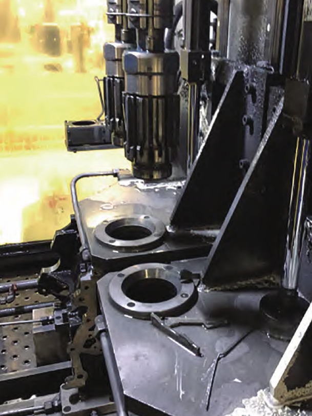
In automotive manufacturing, the demand for lightweight, safe, and environmentally friendly vehicles has increased significantly. Since casting defects directly affect the structural integrity and performance of critical components, nondestructive testing (NDT) has become an essential part of quality control. X-ray radiography is one of the most widely used NDT methods due to its ability to reveal internal defects. The basic principle of X-ray inspection is described by the contrast equation:
$$ \frac{I_T}{I_n} = \frac{\mu \Delta T}{1 + n} $$
where $\mu$ is the linear absorption coefficient, $\Delta T$ is the defect dimension along the X-ray beam direction, and $n$ is the ratio of scattered radiation intensity to primary transmitted intensity. This equation indicates that a detectable defect will produce a certain object contrast when the absorption coefficient differs from the surrounding material and the defect has sufficient size along the beam direction.
Although X-ray inspection is effective, the current industrial practice still relies heavily on manual inspection, which is subjective, labor-intensive, and prone to errors due to operator fatigue. Automated defect detection algorithms based on deep learning have emerged as a promising solution. Nevertheless, these algorithms require a large number of training samples with diverse defect types and appearances. In real production environments, the collection of sufficient defect samples is time-consuming and costly. Therefore, the research on defect image generation algorithms has attracted considerable attention. The purpose is to synthesize realistic defect images that can supplement the training database and improve the robustness of automated inspection algorithms.
This thesis focuses on the generation algorithm for shrinkage cavity defect images in castings. The research is organized into three main stages: the simulation defect image generation stage, the transformation processing stage, and the background fusion stage. In the generation stage, an improved Diamond-Square algorithm is employed to produce random height data. These height data are then mapped to gray values to form the initial simulation defect image. In the transformation stage, a series of image processing operations are applied to make the simulated defect more closely resemble real shrinkage cavity defects. Finally, in the fusion stage, the transformed defect image is fused with a real X-ray background image using a proposed fusion method.
Formation Mechanisms and Classification of Shrinkage Cavity Defects
Shrinkage cavity defects arise from the volumetric contraction of liquid metal during solidification. The contraction process of liquid metal can be divided into three stages: liquid contraction, solidification contraction, and solid contraction. The liquid contraction occurs from the pouring temperature to the liquidus temperature. During this stage, the decrease in volume is reflected only by the lowering of the liquid level in the mold cavity. The solidification contraction stage takes place from the liquidus temperature to the solidus temperature. At this point, a solid shell forms on the outer surface while the inner metal remains liquid. As the inner liquid cools, the interatomic distance decreases, causing a reduction in volume. If the contraction is not compensated by external liquid metal, a concentrated cavity is formed. The total volumetric shrinkage can be expressed as:
$$ V_{total} = V_{liquid} + V_{freeze} + V_{solid} $$
where $V_{liquid}$, $V_{freeze}$, and $V_{solid}$ represent the volume reductions during liquid contraction, solidification contraction, and solid contraction, respectively. The solid contraction stage occurs after complete solidification, and it is mainly related to dimensional changes and the formation of cracks and deformation.
Depending on the position where the defect appears, shrinkage cavities can be classified into several types. Table 1 summarizes the common classification of shrinkage cavity defects.
| Type | Description |
|---|---|
| Open shrinkage cavity | Visible on the surface of the casting, usually at the riser or feeder location. |
| Concave corner shrinkage | Appears at internal concave corners where thermal contraction is constrained. |
| Core surface shrinkage | Occurs on the surface of a core when the molten metal contracts away from the core. |
| Internal shrinkage cavity | Hidden inside the casting, typically at the last solidified regions. |
The American Society for Testing and Materials (ASTM) has established standard reference radiographs for aluminum castings, defining eight severity levels for shrinkage cavity defects. This standard provides a useful benchmark for evaluating both manual and automated defect detection methods. In this work, real shrinkage cavity images collected from wheel hub production lines are used as the reference for algorithm development and evaluation.
Digital Image Features of Shrinkage Cavity Defects
To generate realistic simulation defects, it is essential to first analyze the digital image features of real shrinkage cavity defects. Three categories of features are considered: color features, texture features, and spatial relationship features.
Color Features
Since X-ray images are grayscale images, the color features of these images are equivalent to their gray features. The gray histogram is a straightforward representation of the distribution of pixel intensities. For real shrinkage cavity defect images, the histogram exhibits a distinct peak in the high-intensity region. The gray values are mainly concentrated in the range of 150 to 250, and more specifically in the range of 180 to 220. The gray level contour plot reveals a steep “mountain peak” spatial distribution. The highest gray value appears at the center of the defect, and the gray value decreases gradually from the center to the edge. The difference between the defect region and the background region is significant, and the edge of the defect region shows a “pulse-like” attenuation phenomenon.
Texture Features
Texture features provide valuable information about the spatial arrangement of pixel intensities. In this work, both spectral analysis and statistical analysis are employed to describe the texture of shrinkage cavity defects.
The Fourier spectrum method is used to analyze the periodic and directional properties of the texture. Let the spectrum function be represented in polar coordinates as $S(r, \theta)$. The one-dimensional functions $S(r)$ and $S(\theta)$ are defined as:
$$ S(r) = \sum_{\theta=0}^{\pi} S(r, \theta) $$
$$ S(\theta) = \sum_{r=1}^{O_R} S(r, \theta) $$
where $O_R$ is the radius of a circle centered at the origin. For real shrinkage cavity defects, the spectrum $S(r)$ has a single peak at approximately $r=3$, indicating no obvious periodicity. The spectrum $S(\theta)$ shows strong energy concentrations near $0^\circ$, $90^\circ$, and $180^\circ$, implying that the texture has strong horizontal and vertical orientations.
In addition to the spectral approach, statistical descriptors based on the gray histogram are computed. The key texture measures are the mean, standard deviation, smoothness, and entropy, defined by the following equations:
$$ m = \sum_{i=0}^{L-1} z_i p(z_i) $$
$$ \sigma = \sqrt{\sum_{i=0}^{L-1} (z_i – m)^2 p(z_i)} $$
$$ R = 1 – \frac{1}{1 + \sigma^2} $$
$$ e = -\sum_{i=0}^{L-1} p(z_i) \log_2 p(z_i) $$
where $z_i$ is the gray level, $p(z_i)$ is the histogram probability, and $L$ is the number of gray levels. These measures characterize the average brightness, contrast, smoothness, and complexity of the texture. Table 2 lists the texture measures for two representative real shrinkage cavity defect images, and Table 3 presents the averaged values over 400 real defect samples. These values serve as the evaluation standard for the simulated defects.
| Image | Mean brightness | Mean contrast | Smoothness | Entropy |
|---|---|---|---|---|
| Sample (a) | 206.326 | 22.846 | 0.008 | 5.549 |
| Sample (b) | 187.098 | 20.099 | 0.006 | 6.155 |
| Set | Mean brightness | Mean contrast | Smoothness | Entropy |
|---|---|---|---|---|
| 400 real defects | 195.226 | 19.266 | 0.006 | 6.534 |
Spatial Relationship Features
From the perspective of spatial relationships, shrinkage cavity defects are usually concentrated and hidden in the upper part of the casting interior or in the last solidified regions. They often appear in thick-wall sections, at the intersection of two walls, and near the riser. These locations are called hot spots, where the cooling rate is slow and the metal remains liquid for a longer time. Figure 1 in the original thesis illustrates a shrinkage cavity defect at a hot spot. Understanding these spatial characteristics helps in determining suitable regions for defect placement during the simulation generation process.
Simulation Defect Image Generation Stage
The generation of simulation defect images is the first and most crucial stage of the proposed algorithm. The Diamond-Square algorithm is chosen as the basis for this stage due to its ability to generate random height data with natural-looking mountain-peak structures, which resemble the gray distribution of real shrinkage cavity defects.
Random Midpoint Displacement Method
The random midpoint displacement method is a classical technique for generating fractal Brownian motion. The one-dimensional version can be described as follows. Given a segment with two endpoints having initial height values, the height of the midpoint is set to the average of the two endpoint values plus a random displacement. This process is recursively applied to each sub-segment until the desired level of detail is achieved. The recursive relation is:
$$ X\left(\frac{t_1 + t_2}{2}\right) = \frac{X(t_1) + X(t_2)}{2} + \Delta_n $$
where $\Delta_n$ is a Gaussian random variable with zero mean and variance $\Delta_n^2$. The variance decreases with each iteration according to:
$$ \Delta_n^2 = \frac{k}{2^{2nH}} $$
where $n$ is the iteration count, $k$ is a scale factor, and $H$ is the Hurst exponent. The random midpoint displacement method can be extended to two dimensions to generate height maps.
Diamond-Square Algorithm
The Diamond-Square algorithm, also known as the diamond-square subdivision method, is the most commonly used two-dimensional random midpoint displacement technique. The algorithm begins with a square two-dimensional array of size $(2^n+1) \times (2^n+1)$. Initially, the four corner points of the array are set to random height values in the range $[-1, 1]$. The algorithm then proceeds through two iterative steps: the Diamond step and the Square step.
In the Diamond step, the center point of the square is calculated as the average of the four corner values plus a random displacement. For the four corners with heights $g_A$, $g_B$, $g_C$, and $g_D$, the center height $g_M$ is given by:
$$ g_M = \frac{g_A + g_B + g_C + g_D}{4} + r_M $$
In the Square step, the midpoint of each edge of the square is calculated. For example, the height of the top edge midpoint is computed as the average of the two adjacent corner values and the center value, plus a random displacement:
$$ g_E = \frac{g_A + g_B + g_M}{3} + r_E $$
where $r_E$ is a random displacement that is smaller than the displacement used in the Diamond step. The process is repeated recursively, generating $4^i$ sub-squares after $i$ iterations. The number of squares after $i$ iterations is:
$$ M = 2^{2i}, \quad i \geq 1 $$
Throughout the recursion, the range of the random displacement is gradually decreased to ensure that the surface becomes smoother with increasing resolution.
Improved Diamond-Square Algorithm for Defect Generation
In this work, the original Diamond-Square algorithm is improved to better match the characteristics of real shrinkage cavity defects. The improvement consists of setting a larger random displacement for the center point of the array compared to other points. This increases the probability that the highest elevation data will be concentrated in the central part of the generated image. This modification aligns with the observation that shrinkage cavity defects have their highest gray value at the center and gradually decreasing values toward the edges, forming a “tumor-like” structure with “ribbon-like” edges.
After generating the height data, the values need to be mapped to the grayscale space. The mapping process is as follows. First, the minimum absolute value $d_{min}$ in the two-dimensional array is identified, and all height data are shifted by this value to make them non-negative. Next, the maximum absolute value $d_{max}$ is found, and all shifted values are divided by $d_{max}$ to normalize the data to the range $[0, 1]$. Finally, the normalized values are multiplied by 255 to obtain grayscale values in the range $[0, 255]$. The resulting image is the initial simulation defect image. Figure 4-2 in the original thesis shows several examples of such generated defect images, which appear as cloud-like gray images with white regions representing high elevation areas.
To evaluate the improved algorithm, the grayscale contour plots of the generated images were compared with those produced by the unmodified algorithm. The improved version produces “mountain peaks” that are more concentrated in the center of the image, closely matching the gray distribution of real shrinkage cavity defects. The gray histogram of the generated images also shows high concentration in the range of 150 to 250, which is consistent with real defects.
Simulation Defect Image Transformation Processing Stage
Although the initial simulation defect images share some similarities with real defects, they still differ in terms of contrast and sharpness. Direct fusion of these images with a background image would produce unrealistic results. Therefore, a transformation processing stage is necessary to refine the simulation defect image and make it more closely approximate the real defect appearance.
Histogram Equalization
The first transformation operation is histogram equalization, which is an effective technique for enhancing image contrast. The gray values of the initial simulation defect image are not uniformly distributed; they are mainly concentrated in the high-intensity range of 150 to 250. Histogram equalization redistributes the gray values over the entire range of 0 to 255, thereby enhancing the contrast and making the defect structure more visible.
The theoretical foundation of histogram equalization is based on the concept of information entropy. The entropy $H$ of an image with gray level probabilities $p_i$ is:
$$ H = -\sum_{i=0}^{L-1} p_i \log p_i $$
It can be shown that the entropy is maximized when all gray levels are equally probable. Histogram equalization approximates this condition by transforming the input gray levels using the cumulative distribution function. After the transformation, the image has a more uniform gray distribution, which improves the subjective visual quality and facilitates subsequent processing steps.
Thresholding Using Improved Otsu Method
After histogram equalization, a thresholding operation is applied to separate the defect region from the background and to remove the lower-intensity parts of the defect. The original Otsu method, also known as the maximum inter-class variance method, is an adaptive threshold selection algorithm. The optimal threshold $k^*$ is obtained by maximizing the between-class variance:
$$ \sigma_B^2 = \omega_0 (\mu_0 – \mu_T)^2 + \omega_1 (\mu_1 – \mu_T)^2 $$
where $\omega_0$ and $\omega_1$ are the probabilities of the two classes, $\mu_0$ and $\mu_1$ are their mean gray values, and $\mu_T$ is the total mean gray value. The optimal threshold is given by:
$$ k^* = \arg \max_{k \in [1, L]} \sigma_B^2(k) $$
In the proposed algorithm, an improvement is made to the original Otsu method by introducing a dynamic coefficient $\sigma$ with a range of $[1.2, 1.5]$. The final threshold $k$ is computed as:
$$ k = k^* \times \sigma $$
All pixels with gray values below $k$ are set to $k$. The dynamic coefficient introduces a certain randomness into the threshold, making the filtering process more flexible and ensuring that the remaining defect parts are more diverse and arbitrary. This helps to simulate the natural variability of real shrinkage cavity defects.
Gray Stretching
After thresholding, gray stretching is applied to enhance the contrast of the remaining defect region. Gray stretching uses a linear scaling function to expand the range of gray values. The transformation is given by:
$$ g(i,j) = \left( \frac{f(i,j) – f_{min}}{f_{max} – f_{min}} \right) \times 255 $$
where $f(i,j)$ and $g(i,j)$ are the input and output pixel values at coordinate $(i,j)$, and $f_{min}$ and $f_{max}$ are the minimum and maximum gray values of the input image, respectively. This operation maps the gray value range of the defect region from $[k, f_{max}]$ to $[0, 255]$, thereby increasing the dynamic range and improving the visual contrast.
Gaussian Filtering
Finally, Gaussian filtering is applied to smooth the defect region and suppress noise. The two-dimensional Gaussian filter is defined as:
$$ G(x,y) = \frac{1}{2\pi\sigma^2} \exp\left( -\frac{x^2 + y^2}{2\sigma^2} \right) $$
where $\sigma^2$ is the variance of the Gaussian function. The Gaussian filter performs a weighted average of the pixel values in the neighborhood of each pixel. This operation softens the sharp changes in the defect region, making the simulated defect look more natural. After Gaussian filtering, the defect image is once again subjected to thresholding, gray stretching, and Gaussian filtering to further refine the defect appearance and improve the fusion quality. The final transformed defect images are shown in the experimental section of the original thesis.
Background Fusion Stage
The background fusion stage aims to fuse the transformed simulation defect image with a real X-ray background image. This stage is critical because the fusion result should be visually realistic and the fused defect should blend seamlessly with the background.
Image Fusion Levels and Algorithms
Image fusion can be performed at three different levels: pixel level, feature level, and decision level. Pixel-level fusion operates directly on the image data and preserves the maximum amount of information. Feature-level fusion processes the extracted features from the source images and offers a good trade-off between information preservation and computational efficiency. Decision-level fusion, the highest level, combines the decisions from multiple sources and has the best real-time performance but suffers from significant information loss. For this work, pixel-level fusion is selected because it is the most suitable for preserving the fine details of the defect image.
Common pixel-level fusion algorithms include weighted averaging, maximum/minimum pixel selection, principal component analysis (PCA), and pyramid-based methods. In the proposed approach, a novel fusion algorithm is developed, specifically designed for the characteristics of shrinkage cavity defect images and cast X-ray background images.
Proposed Fusion Algorithm
The proposed fusion algorithm is described as follows. Let $D$ be the simulation defect image and $F$ be the real X-ray background image. The algorithm consists of the following steps:
Step 1: Compute the maximum gray value of the background image $F$, denoted as $\max\_F$. The transformation upper limit $T$ is then calculated as:
$$ T = \frac{255}{5 \times \max\_F} $$
Step 2: Compute the maximum and minimum gray values of the simulation defect image $D$, denoted as $D_{max}$ and $D_{min}$, respectively.
Step 3: Map all pixel values of $D$ to the interval $[1, T]$ using the following equation:
$$ M(i,j) = \left( \frac{D(i,j) – D_{min}}{D_{max} – D_{min}} \right) \cdot (T – 1) + 1 $$
where $M(i,j)$ is the mapped value at coordinate $(i,j)$.
Step 4: Multiply the mapped matrix $M$ with the background image $F$ pixel by pixel to obtain the final fused image $R$:
$$ R(i,j) = M(i,j) \cdot D(i,j) $$
The fusion algorithm ensures that the simulation defect is naturally embedded into the background image, avoiding the appearance of a defect “floating” on the surface. This is essential for generating realistic simulation samples that can be used to train automated defect detection algorithms.
Experimental Results and Evaluation
Experimental Platform
The experiments were conducted in a software environment consisting of Microsoft Visual Studio 2010 with C++ and MATLAB. The hardware platform was an Intel Core i5-2520M CPU at 2.50 GHz with 4 GB of RAM. The Diamond-Square algorithm was implemented in the C++ environment, while the transformation processing and background fusion operations were implemented in MATLAB. The defect detection evaluation was performed using a deep learning-based detection algorithm.
Results of Simulation Defect Generation
Figure 4-2 in the original thesis shows several simulation defect images generated by the improved Diamond-Square algorithm. The generated images have a cloud-like appearance with the defect region concentrated in the center. The grayscale contour plots confirm that the high-gray-value region is concentrated at the center of the image, which matches the observation of real shrinkage cavity defects. Compared with the unmodified Diamond-Square algorithm, the improved version produces defects with a more prominent central peak, as illustrated by the contour plots in the experimental section. The gray histograms of the generated images also show that the gray values are mainly concentrated in the high-intensity range of 150 to 250, which is consistent with real defect images.
Results of Transformation Processing
The transformation processing stage significantly improves the quality of the simulation defect images. After histogram equalization, the contrast of the defect region is greatly enhanced, and the gray distribution becomes more uniform over the entire 0 to 255 range. The improved Otsu thresholding filters out the low-gray-value parts of the defect, leaving only the core region. Gray stretching further increases the dynamic range of the remaining defect region, and Gaussian filtering smooths the sharp boundaries. Table 4 lists the texture measures of the fused images before the second round of transformation processing. The values show some deviation from the real defect statistics in Table 3, indicating that the initial fused defects were too large and had higher brightness and contrast than real defects.
| Image | Mean brightness | Mean contrast | Smoothness | Entropy |
|---|---|---|---|---|
| Sample (b) | 215.626 | 22.237 | 0.017 | 6.439 |
| Sample (f) | 219.556 | 28.223 | 0.015 | 6.162 |
After applying the second round of thresholding, gray stretching, and Gaussian filtering, the final simulation defect images were obtained. These images were then fused with the real X-ray background using the proposed fusion algorithm. The final fused images are shown in Figure 4-14 of the original thesis.
Results of Background Fusion and Feature Comparison
Figure 4-15 in the original thesis presents a detailed feature analysis of the final fused defect images. The gray histograms of the simulated defects show a sharp peak in the high-intensity region, similar to real defects. The grayscale contour plots reveal a steep mountain-like spatial distribution, with the highest gray value at the center and gradually decreasing values toward the edges. The Fourier spectrum analysis shows that the energy is concentrated in the horizontal and vertical directions, consistent with real defect images. The $S(r)$ curve has a single peak at $r=3$, and the $S(\theta)$ curve shows strong energy near $0^\circ$, $90^\circ$, and $180^\circ$, further confirming the similarity.
Table 5 lists the texture measures of two final fused defect images, and Table 6 presents the averaged values over 400 fused images. Comparing Table 6 with Table 3, it is evident that the simulated defects closely match the real defects in terms of mean brightness, contrast, smoothness, and entropy. This indicates that the proposed generation algorithm and the fusion algorithm are effective in producing realistic shrinkage cavity defect images.
| Image | Mean brightness | Mean contrast | Smoothness | Entropy |
|---|---|---|---|---|
| Sample (a) | 191.958 | 19.153 | 0.006 | 6.238 |
| Sample (b) | 196.604 | 18.752 | 0.005 | 6.165 |
| Set | Mean brightness | Mean contrast | Smoothness | Entropy |
|---|---|---|---|---|
| 400 fused images | 193.219 | 18.863 | 0.006 | 6.235 |
Defect Detection Results
To further evaluate the effectiveness of the generated simulation defects, a deep learning-based casting defect detection algorithm was employed. The algorithm uses a Faster R-CNN network for defect detection and classification. The experiment was conducted on 80 fused images containing simulated shrinkage cavity defects. The detection results show that all simulated defects were successfully detected and identified as shrinkage cavity defects, with an average recognition probability of 89.2%. The high recognition rate demonstrates that the generated simulation defects are highly similar to real shrinkage cavity defects and can be effectively used as training samples for automated defect detection algorithms.
Conclusion and Future Work
In this thesis, a comprehensive algorithm for generating shrinkage cavity defect images is proposed. The algorithm consists of three main stages: simulation defect image generation, transformation processing, and background fusion. The improved Diamond-Square algorithm successfully generates random height data with a central peak structure, which is then transformed into grayscale images resembling real defects. The transformation processing stage, including histogram equalization, improved Otsu thresholding, gray stretching, and Gaussian filtering, refines the defect appearance and makes it more realistic. The proposed fusion algorithm seamlessly embeds the simulation defect into real X-ray background images. Subjective and objective evaluations confirm that the generated fusion images closely match the gray and texture features of real shrinkage cavity defects. The deep learning-based detection experiment further validates the effectiveness of the proposed algorithm, with an average recognition rate of 89.2%.
There are several directions for future research. First, the proposed algorithm can be extended to generate other types of casting defects, such as shrinkage sponge defects, gas holes, and inclusion defects. Second, the algorithm could be accelerated using GPU computation to improve real-time performance. Third, a statistical study of the spatial distribution of real defects could be conducted to enhance the randomness and validity of the defect placement in the background fusion stage. These improvements would further increase the practicality and versatility of the defect image generation approach, contributing to the advancement of automated casting defect detection systems.