
In this work, I investigate the high-precision modeling of wax viscosity during wax pattern injection forming for investment casting, with particular attention to aerospace titanium alloy structural components. I treat the wax as a non-Newtonian fluid that exhibits shear-thinning behavior, and I show that the Cross-WLF model can describe the coupled dependence of viscosity on shear rate and temperature. I also emphasize that the same kind of viscosity-driven dimensional fidelity problem appears in evaporative pattern casting, where pattern deformation and collapse behavior must be controlled before metal pouring. Although my experimental focus is wax injection for investment casting, the modeling strategy I propose is relevant to evaporative pattern casting because both processes require a reliable constitutive description of a pattern material whose flow and solidification history determines final dimensional accuracy.
The motivation for this study is straightforward. Titanium alloy structural components used in aerospace applications must satisfy extremely tight dimensional tolerances, and investment casting is one of the most important near-net-shape manufacturing routes for such components. In the investment casting chain, the wax pattern is not a temporary artifact of secondary importance; its dimensions, surface quality, and structural stability directly determine the final casting precision. The wax pattern is produced by injection molding, and traditional process control still relies heavily on experience-based trial and error. In many industrial settings, engineers adjust injection temperature, pressure, holding time, and cooling conditions over three to five rounds of trials. This approach is slow, expensive, and poorly suited to complex titanium alloy components. Numerical simulation can reduce trial cycles by predicting filling, cooling, shrinkage, and warpage, but the predictive accuracy of simulation depends critically on the accuracy of the material viscosity model. In evaporative pattern casting, the same logic applies to the foam pattern: if the pattern material model is inaccurate, simulation cannot reliably predict pattern dimensions or defect formation.
I selected a commercial wax designated Kc-4017b as the research material. Its density is 0.95 g/cm³, its drop point is 94 °C, and its softening point is 79 °C. The wax displays clear shear-thinning behavior: at a fixed temperature, the apparent viscosity decreases rapidly at low shear rates and then approaches a plateau at higher shear rates. Temperature also has a strong effect; at the same shear rate, a higher temperature produces a lower viscosity. Therefore, a viscosity model that considers only shear rate or only temperature is insufficient. The Cross-WLF model combines a Cross shear-thinning term with a Williams-Landel-Ferry temperature-sensitive term and can describe both effects simultaneously. This is why I adopted Cross-WLF as the constitutive framework for the wax. The same reasoning is useful in evaporative pattern casting, where the flow and softening of the pattern material are also controlled by coupled thermal and deformation histories.
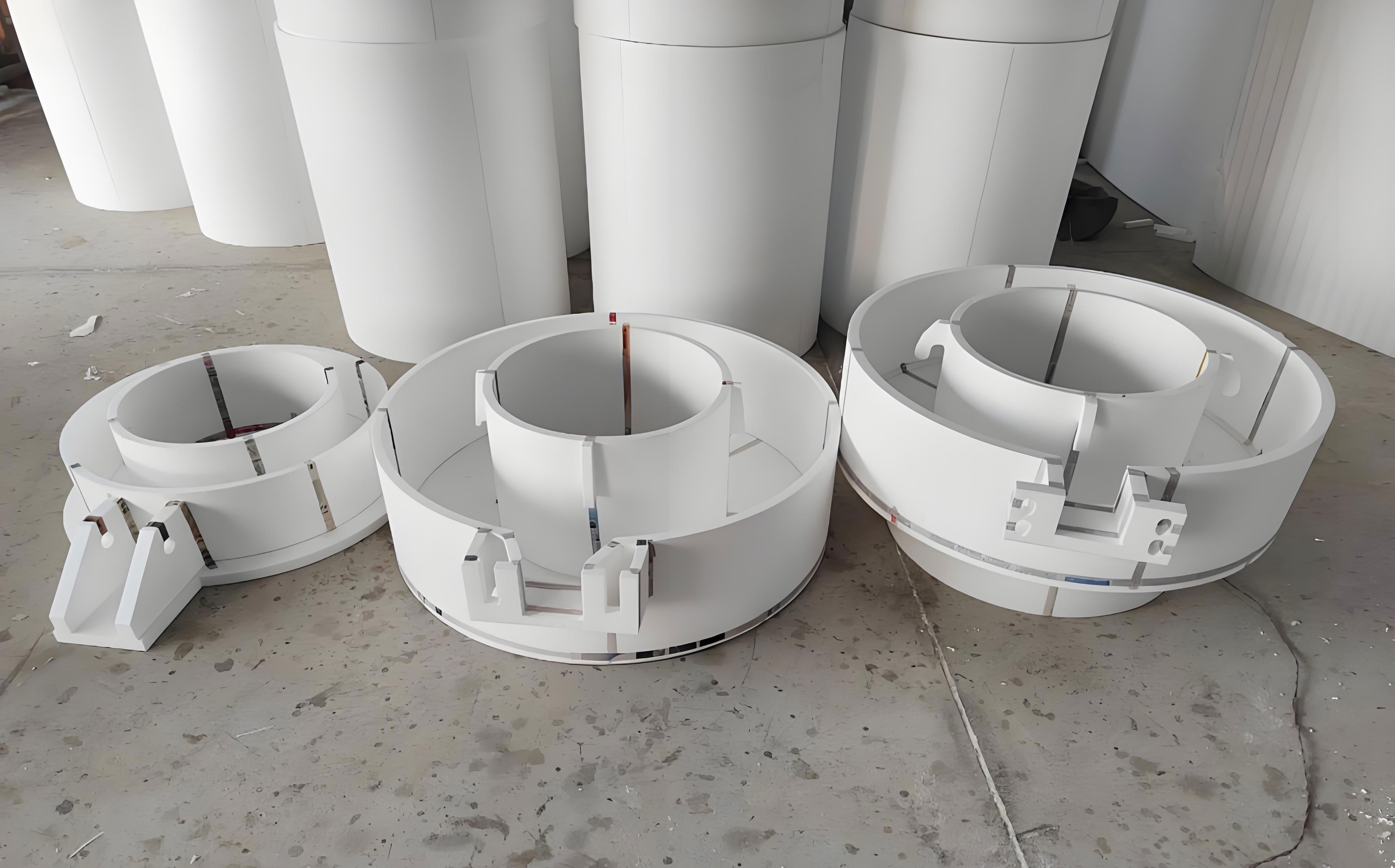
I designed an annular stepped wax pattern to represent the complex ring-shaped and variable-wall-thickness features often found in aerospace titanium alloy structural components. The pattern contains multiple wall thicknesses, which makes the filling process sensitive to viscosity changes. The injection experiments were performed on an MPI-25 t wax injection machine. The wax temperature was set to 65 °C, the mold temperature was 25 °C, the holding pressure was 1 MPa, and the holding time was 60 s. The gate diameter was 8 mm. To ensure repeatability, I repeated the injection experiment five times under the same conditions. After injection, I used blue light scanning to measure the displacement and dimensional changes of the wax pattern. These measured data were later compared with numerical simulation results. In parallel, I constructed a three-dimensional model of the annular stepped wax pattern and imported it into Moldflow for numerical simulation. The mesh was a double-layer mesh with a global edge length of 2 mm. The analysis sequence was set to cooling-filling-packing-warping, so that the full injection forming history could be captured. The boundary heat transfer coefficient between the wax and the mold was set to 2 500 W/(m²·K). The Cross-WLF viscosity parameters obtained from my modeling method were imported into the Moldflow database to improve simulation accuracy.
| Property or Parameter | Value | Unit |
|---|---|---|
| Wax material | Kc-4017b | — |
| Density | 0.95 | g/cm³ |
| Drop point | 94 | °C |
| Softening point | 79 | °C |
| Rheological behavior | Non-Newtonian, shear thinning | — |
| Temperature range studied | 60–64 | °C |
The Cross-WLF model is defined by a set of equations that I used throughout the parameter identification process. The shear-rate dependence is described by the Cross model:
$$ \eta(\dot{\gamma}, T) = \frac{\eta_0(T)}{1 + \left( \frac{\eta_0(T)\dot{\gamma}}{\tau^*} \right)^{1-n}} $$
Here, \(\eta\) is the apparent viscosity, \(\eta_0\) is the zero-shear viscosity, \(\dot{\gamma}\) is the shear rate, \(\tau^*\) is a characteristic relaxation parameter, and \(n\) is the non-Newtonian index. When \(n < 1\), the material exhibits shear thinning. The zero-shear viscosity is described by the WLF equation:
$$ \eta_0(T) = D_1 \exp\left[-\frac{A_1 (T – T^*)}{A_2 + (T – T^*)}\right] $$
The reference temperature \(T^*\) is related to pressure by:
$$ T^* = D_2 + D_3 p $$
In these expressions, \(D_1\) is the zero-shear viscosity coefficient at the reference temperature, \(D_2\) is the glass transition temperature at low pressure, \(D_3\) is the pressure coefficient, and \(A_1\) and \(A_2\) are WLF parameters. For the wax studied here, \(D_3\) is taken as zero because the material is a small-molecule organic non-Newtonian fluid and the pressure dependence is negligible compared with the temperature and shear-rate effects. Combining the Cross and WLF equations gives the full Cross-WLF form:
$$ \eta(\dot{\gamma}, T, p) = \frac{D_1 \exp\left[-\frac{A_1 (T – D_2 – D_3 p)}{A_2 + (T – D_2 – D_3 p)}\right]}{1 + \left( \frac{D_1 \exp\left[-\frac{A_1 (T – D_2 – D_3 p)}{A_2 + (T – D_2 – D_3 p)}\right] \dot{\gamma}}{\tau^*} \right)^{1-n}} $$
This model contains seven key parameters: \(n\), \(\tau^*\), \(D_1\), \(D_2\), \(D_3\), \(A_1\), and \(A_2\). The identification of these parameters is a high-dimensional nonlinear optimization problem. In the context of evaporative pattern casting, a similar parameter identification problem arises when the deformation and flow of the pattern material must be described under coupled thermal and mechanical loads.
| Symbol | Meaning | Role in Cross-WLF Model |
|---|---|---|
| \(\eta\) | Apparent viscosity | Primary output |
| \(\eta_0\) | Zero-shear viscosity | Temperature-dependent baseline |
| \(\dot{\gamma}\) | Shear rate | Shear-thinning input |
| \(\tau^*\) | Characteristic relaxation parameter | Controls transition from Newtonian plateau |
| \(n\) | Non-Newtonian index | Controls shear-thinning slope |
| \(D_1\) | Reference zero-shear viscosity coefficient | WLF scale factor |
| \(D_2\) | Low-pressure glass transition temperature | WLF reference temperature |
| \(D_3\) | Pressure coefficient | Pressure shift; set to zero here |
| \(A_1\) | WLF temperature sensitivity parameter | Controls temperature dependence |
| \(A_2\) | WLF temperature offset parameter | Controls curvature of temperature response |
Traditional parameter fitting for Cross-WLF models often uses a simple least-squares method. I found that this approach is inadequate for wax because the model is strongly nonlinear and the parameters are coupled. The simple least-squares method relies mainly on first-order gradient information, so it cannot easily capture second-order coupling effects among parameters. As a result, it is prone to local minima. It is also sensitive to the initial guess. When the initial parameter set is far from the physically reasonable range, the fitting error increases and the model becomes poorly adapted to the experimental data. Newton’s method is another common choice. It uses both the gradient and the Hessian matrix to construct a quadratic approximation of the objective function. The iteration formula is:
$$ \theta_{k+1} = \theta_k – H^{-1}(\theta_k) \nabla L(\theta_k) $$
Here, \(\theta\) is the parameter vector, \(\nabla L\) is the gradient, and \(H\) is the Hessian matrix. Newton’s method can converge quickly near the optimum, but it has two serious drawbacks. First, computing the Hessian matrix and its inverse has a complexity of \(O(n^3)\), which becomes expensive for a seven-parameter model. Second, if the Hessian matrix is singular or ill-conditioned, for example when the condition number \(\kappa(H) > 10^6\), Newton’s method may become numerically unstable, oscillatory, or non-convergent. These problems are especially severe for wax viscosity data, which vary strongly with temperature and shear rate. The same numerical challenges can appear in the material modeling of evaporative pattern casting, where foam deformation and collapse behavior are also nonlinear and strongly coupled.
To overcome these limitations, I proposed a quasi-Newton method that integrates automatic differentiation and SVD regularization. The core idea is to avoid direct computation of the Hessian matrix and instead construct a positive-definite approximation of the Hessian inverse. I use gradient information from successive iterations and update the inverse Hessian approximation by the BFGS formula. Automatic differentiation is used to obtain gradients with high numerical accuracy, and SVD regularization is used to handle ill-conditioning. When the condition number of the approximate Hessian exceeds \(10^6\), small singular values are truncated to prevent numerical explosion. This reduces the computational complexity from \(O(n^3)\) to \(O(n^2)\). The method therefore addresses the accuracy limitations of simple least squares and the computational and stability limitations of Newton’s method.
The objective function I minimized is the sum of squared differences between the measured viscosity and the model prediction:
$$ L(\theta) = \sum_{i=1}^{N} \left[ \eta_i^{\exp} – \eta_i^{\text{model}}(\dot{\gamma}_i, T_i; \theta) \right]^2 $$
The parameter vector is:
$$ \theta = \left[ n,\ \tau^*,\ D_1,\ D_2,\ A_1,\ A_2 \right]^T $$
Because \(D_3\) is zero, it is not included as an active optimization variable. The quasi-Newton update is written as:
$$ \theta_{k+1} = \theta_k – \alpha_k H_k^{-1} \nabla L(\theta_k) $$
where \(k\) is the iteration index, \(\alpha_k\) is the step length, and \(H_k^{-1}\) is the approximate inverse Hessian updated by the BFGS formula:
$$ H_{k+1}^{-1} = \left(I – \frac{s_k y_k^T}{y_k^T s_k}\right) H_k^{-1} \left(I – \frac{y_k s_k^T}{y_k^T s_k}\right) + \frac{s_k s_k^T}{y_k^T s_k} $$
In this formula, \(s_k = \theta_{k+1} – \theta_k\) is the parameter change and \(y_k = \nabla L(\theta_{k+1}) – \nabla L(\theta_k)\) is the gradient change. The BFGS update preserves positive definiteness, which is important for stable descent. The step length is determined by the Armijo condition:
$$ L(\theta_k + \alpha_k p_k) \le L(\theta_k) + c_1 \alpha_k \nabla L(\theta_k)^T p_k $$
where \(p_k = -H_k^{-1} \nabla L(\theta_k)\) is the search direction and \(c_1 = 0.01\). This condition ensures sufficient decrease in the objective function and improves global convergence behavior. When the approximate Hessian matrix \(A\) is close to singular, I apply singular value decomposition:
$$ A = U \Sigma V^T $$
with
$$ \Sigma = \text{diag}(\sigma_1, \sigma_2, \dots, \sigma_n) $$
The inverse is computed as:
$$ A^{-1} \approx V \Sigma_{\epsilon}^{-1} U^T $$
where small singular values are truncated according to:
$$ \sigma_i < \epsilon \sigma_{\max} \Rightarrow \sigma_i^{-1} = 0 $$
This SVD regularization step prevents numerical explosion and stabilizes the iteration. Automatic differentiation provides the gradient vector:
$$ \nabla L(\theta) = \left( \frac{\partial L}{\partial n}, \frac{\partial L}{\partial \tau^*}, \frac{\partial L}{\partial D_1}, \frac{\partial L}{\partial D_2}, \frac{\partial L}{\partial A_1}, \frac{\partial L}{\partial A_2} \right)^T $$
I implemented this workflow and compared it with simple least squares. The comparison was performed at 60 °C, 62 °C, and 64 °C. For each temperature, I evaluated the coefficient of determination:
$$ R^2 = 1 – \frac{\sum_{i=1}^{N} (y_i – \hat{y}_i)^2}{\sum_{i=1}^{N} (y_i – \bar{y})^2} $$
The fitted Cross-WLF parameters are summarized in the table below. The quasi-Newton method produced \(n = 0.62\), \(\tau^* = 0.61\), \(D_1 = 1.08 \times 10^{17}\), \(D_2 = 263.85\), \(A_1 = 55.85\), and \(A_2 = 51.38\). The simple least-squares method produced \(n = 0.72\), \(\tau^* = 0.11\), \(D_1 = 1.77 \times 10^{17}\), \(D_2 = 256.66\), \(A_1 = 78.13\), and \(A_2 = 99.98\). These differences are not merely numerical; they reflect the different abilities of the two methods to capture the coupled nonlinear rheology of the wax. The quasi-Newton parameters produced a more physically consistent transition from the low-shear plateau to the shear-thinning regime.
| Parameter | Quasi-Newton Method | Simple Least-Squares Method |
|---|---|---|
| \(n\) | 0.62 | 0.72 |
| \(\tau^*\) | 0.61 | 0.11 |
| \(D_1\) | \(1.08 \times 10^{17}\) | \(1.77 \times 10^{17}\) |
| \(D_2\) | 263.85 | 256.66 |
| \(D_3\) | 0 | 0 |
| \(A_1\) | 55.85 | 78.13 |
| \(A_2\) | 51.38 | 99.98 |
The fitting results show that both methods can reproduce the general shear-thinning trend, but the quasi-Newton method produces a much better match to the experimental data. At low shear rates, the difference between the two methods is relatively small. As the shear rate increases, the deviation of the simple least-squares method becomes larger, while the quasi-Newton curve remains close to the experimental points. This behavior is consistent with the fact that the quasi-Newton method captures second-order parameter coupling and avoids the local minima that affect first-order least-squares fitting. The advantage is more pronounced at 60 °C, where the wax molecules are more entangled and the viscosity is more sensitive to shear rate. At 62 °C and 64 °C, the molecular mobility increases, the overall viscosity decreases, and the sensitivity to shear rate becomes somewhat weaker, but the quasi-Newton method still maintains higher accuracy.
| Temperature | \(R^2\) Quasi-Newton | \(R^2\) Least Squares | Improvement |
|---|---|---|---|
| 60 °C | 0.989 | 0.901 | +0.088 |
| 62 °C | 0.989 | 0.901 | +0.088 |
| 64 °C | 0.989 | 0.901 | +0.088 |
| Overall | 0.989 | 0.901 | +0.088 |
The residual analysis provides further evidence. I examined the residual distribution as a function of shear rate and temperature. The quasi-Newton method produced a relatively flat residual surface with small, uniformly distributed residuals. The least-squares method produced localized peaks, which indicate that certain combinations of shear rate and temperature are poorly fitted. In histogram form, the quasi-Newton residuals are concentrated near zero, whereas the least-squares residuals are more broadly scattered and contain a larger number of high-magnitude errors. This residual behavior matters for process simulation because large local errors in viscosity can translate into incorrect filling patterns, incorrect pressure transmission, and inaccurate warpage prediction. In evaporative pattern casting, similar local errors in material properties can lead to incorrect predictions of pattern deformation and coating failure.
| Residual Metric | Quasi-Newton Method | Least-Squares Method |
|---|---|---|
| Mean residual magnitude | Low | Higher |
| Standard deviation | Small | Large |
| Maximum absolute residual | Small | Large |
| Distribution shape | Concentrated near zero | Broad and scattered |
| Surface smoothness | Flat and uniform | Local peaks and valleys |
After obtaining the Cross-WLF parameters, I imported them into Moldflow and performed the full injection forming simulation. The filling stage was analyzed first. When the melt contacts the mold wall, the temperature drops rapidly toward the mold temperature. Only the melt front remains at a relatively high temperature as it advances. The simulated melt-front temperature was 62 °C, which agrees with the specified temperature and confirms that the thermal boundary conditions were reasonable. The viscosity field showed a similar trend. Near the wall, the viscosity increased sharply because of rapid cooling. At the melt front, the viscosity remained lower. With the quasi-Newton parameters, the melt-front viscosity was 1.36 Pa·s. With the least-squares parameters, it was 0.86 Pa·s. The quasi-Newton value is more consistent with the experimental viscosity data, which supports the reliability of the proposed modeling method.
| Simulation Quantity | Quasi-Newton Parameters | Least-Squares Parameters |
|---|---|---|
| Melt-front temperature | 62 °C | 62 °C |
| Melt-front viscosity | 1.36 Pa·s | 0.86 Pa·s |
| Wall viscosity | Sharp increase toward solid-like value | Sharp increase toward solid-like value |
| Filling trend | Stable, physically consistent | Less consistent with measured viscosity |
The cooling stage is closely linked to dimensional accuracy. The wax pattern shrinks during cooling, and the uniformity of shrinkage depends on the temperature field and the viscosity evolution. A higher viscosity, such as that predicted by the quasi-Newton model, corresponds to stronger molecular entanglement and a more gradual rearrangement of molecular chains during cooling. This slower contraction behavior makes the temperature field and shrinkage field evolve more synchronously. As a result, the cross-sectional temperature gradients are smaller, and the warpage value is slightly lower than that predicted using the least-squares parameters. This is important because warpage is one of the main sources of dimensional error in wax patterns. The same principle applies to evaporative pattern casting, where the dimensional stability of the pattern during cooling and storage affects the final casting dimensions.
I validated the simulation by comparing it with actual injection experiments. After injection and holding, the wax pattern was removed and allowed to cool. Blue light scanning was used to record the displacement field. The simulated average volumetric shrinkage field was then compared with the measured displacement field. The stepped geometry caused large differences in volumetric shrinkage among different regions. The regions where the shrinkage rate changed abruptly were identified as high-risk zones for dimensional deviation. In the simulation, abrupt changes appeared on the second-step surface and near the gate. In the blue light scanning results, displacement mutations appeared at the same locations. The trend of dimensional deviation was therefore consistent between simulation and experiment. The physical wax pattern also showed shrinkage marks at the corresponding positions. These observations confirm that the viscosity model obtained by the quasi-Newton method provides reliable parameters for numerical simulation.
| Validation Aspect | Simulation Result | Experimental Observation |
|---|---|---|
| Shrinkage mutation location | Second-step surface and gate region | Same regions |
| Displacement trend | Localized突变 and steep gradient | Consistent displacement突变 |
| Visible shrinkage marks | Predicted by shrinkage field | Observed on physical wax pattern |
| Overall agreement | High | High |
The broader significance of this work is that it fills a gap in material databases for wax-based materials. Moldflow and similar commercial software packages often contain rheological data for conventional thermoplastic polymers, but they lack reliable Cross-WLF parameters for paraffin wax and wax-based composites. Without such parameters, simulation of wax injection forming cannot be accurately performed. My method provides a practical route to obtain these parameters. It also provides a template for other pattern materials, including those used in evaporative pattern casting. In evaporative pattern casting, the pattern material must maintain dimensional fidelity during molding, coating, storage, and pouring. A high-quality viscosity model is necessary to simulate the pattern-forming stage and to predict how the pattern will deform before it is vaporized by the molten metal.
There are several reasons why the quasi-Newton method performs better than simple least squares. First, the Cross-WLF model is not linear in its parameters. The parameters \(n\), \(\tau^*\), \(D_1\), \(D_2\), \(A_1\), and \(A_2\) interact strongly. For example, changing \(n\) changes the slope of the shear-thinning region, while changing \(\tau^*\) shifts the transition point. Changing \(D_1\), \(A_1\), and \(A_2\) simultaneously changes the zero-shear viscosity curve. A first-order method cannot easily separate these coupled effects. Second, the experimental viscosity data cover multiple temperatures and shear rates. The objective function therefore has a complex landscape with valleys and local minima. The BFGS update accumulates curvature information and builds a better local quadratic model, which helps the optimizer move toward the global optimum. Third, automatic differentiation provides accurate gradients, which reduces numerical error in the gradient calculation. Fourth, SVD regularization prevents instability when the Hessian approximation becomes ill-conditioned. These four factors together explain the higher \(R^2\) and the more uniform residuals.
| Method | Information Used | Computational Complexity | Main Weakness | Performance for Wax Cross-WLF |
|---|---|---|---|---|
| Simple least squares | First-order gradient | Low | Local minima; sensitive to initial guess | \(R^2 = 0.901\) |
| Newton’s method | Gradient and Hessian | \(O(n^3)\) | Singular or ill-conditioned Hessian; high cost | Not used as final model |
| Quasi-Newton with BFGS | Gradient and curvature approximation | \(O(n^2)\) | Requires good gradient and regularization | \(R^2 = 0.989\) |
| Proposed AD + SVD + BFGS | Automatic gradients, truncated SVD, BFGS update | \(O(n^2)\) | Implementation is more complex | Best accuracy and stability |
The physical interpretation of the fitted parameters is also important. The non-Newtonian index \(n = 0.62\) indicates pronounced shear thinning. The relaxation parameter \(\tau^* = 0.61\) Pa indicates the shear stress scale at which the transition from Newtonian-like behavior to shear-thinning behavior occurs. The low value of \(\tau^*\) suggests that the transition occurs at relatively low shear rates, which is consistent with the experimental data. The WLF parameters \(A_1 = 55.85\) and \(A_2 = 51.38\) describe the temperature sensitivity. The fitted \(D_2 = 263.85\) K corresponds to a reference temperature well below the experimental range, which is physically reasonable for a wax that softens near 79 °C. The pressure coefficient \(D_3\) is set to zero because the viscosity measurements were performed at low pressure and the wax is a small-molecule material. If the process pressure were much higher, \(D_3\) could become important, but for wax injection forming at the studied conditions, the simplification is justified.
I also considered the sensitivity of the simulation to the viscosity parameters. A small change in \(n\) or \(\tau^*\) affects the shear-thinning transition and therefore changes the filling pattern. A small change in \(D_1\), \(A_1\), or \(A_2\) shifts the temperature-dependent viscosity baseline and changes the cooling-stage shrinkage. Because the quasi-Newton method fits all parameters simultaneously, it avoids the inconsistent parameter combinations that can arise when parameters are fitted sequentially. Sequential fitting is common in simple least-squares workflows, but it can produce a good fit at one temperature and a poor fit at another. The simultaneous approach used here produces a parameter set that is consistent across the full temperature and shear-rate range. This is especially important for transient processes such as injection molding, where the material experiences a wide range of temperatures and shear rates during a single cycle.
| Parameter | Effect on Viscosity | Effect on Simulation |
|---|---|---|
| \(n\) | Controls shear-thinning slope | Affects filling pattern and pressure drop |
| \(\tau^*\) | Controls transition from plateau to shear thinning | Affects melt-front advancement |
| \(D_1\) | Scales zero-shear viscosity | Affects overall pressure and holding stage |
| \(D_2\) | Sets reference temperature | Affects temperature sensitivity |
| \(A_1\) | Controls strength of temperature dependence | Affects cooling-stage viscosity rise |
| \(A_2\) | Controls curvature of temperature response | Affects shrinkage uniformity |
| \(D_3\) | Pressure dependence | Negligible at low pressure for this wax |
The numerical simulation results also revealed the importance of the gate region. In the annular stepped wax pattern, the gate is a location where the flow field changes rapidly. The shear rate near the gate is high, and the temperature field is strongly affected by the hot melt entering the cavity. The quasi-Newton parameters produced a more realistic viscosity distribution near the gate, which in turn produced a more realistic pressure field. The least-squares parameters produced a lower melt-front viscosity, which would lead to an overprediction of flowability and an underprediction of pressure loss. Such errors can cause the simulation to predict complete filling when the actual mold might short-shot, or to predict lower warpage when the actual part may warp more severely. In evaporative pattern casting, inaccurate flow and deformation predictions can similarly lead to incorrect pattern dimensions and coating defects.
The use of blue light scanning was essential for validation. Blue light scanning provides a dense displacement field over the wax pattern surface, which allows a direct comparison with the simulated warpage and shrinkage fields. I did not rely only on average dimensions; I compared the spatial pattern of displacement. The agreement in the mutation regions was particularly convincing. If the viscosity model were inaccurate, the simulated shrinkage field would not show the same localization. The fact that the simulated and measured mutation regions coincide indicates that the model captures the coupled thermal-mechanical behavior of the wax. This gives confidence that the proposed method can be used for process optimization, not only for offline parameter fitting.
There are several practical benefits of this work. First, it reduces the need for repeated trial injections. By using a reliable viscosity model, engineers can explore the process window numerically before cutting metal or modifying the mold. Second, it improves the accuracy of warpage prediction, which is critical for complex titanium alloy components. Third, it provides a general framework for fitting Cross-WLF parameters for other waxes and pattern materials. Fourth, it makes the simulation database more complete for wax-based investment casting. Fifth, it offers a methodological bridge to evaporative pattern casting, where pattern material modeling is equally important. In evaporative pattern casting, the pattern is made of foam, but the same principles of shear-thinning behavior, temperature sensitivity, and nonlinear parameter identification apply during the pattern molding stage.
| Benefit | Description | Relevance to Evaporative Pattern Casting |
|---|---|---|
| Reduced trial cycles | Fewer physical injection trials | Fewer pattern molding trials |
| Improved warpage prediction | Better shrinkage and displacement fields | Better pattern dimensional control |
| General fitting framework | Applicable to other waxes and polymers | Applicable to foam pattern materials |
| Database completion | Fills missing Cross-WLF wax data | Supports pattern material databases |
| Numerical stability | SVD regularization and BFGS update | Handles ill-conditioned material models |
The limitations of this study should also be noted. The experimental temperature range was 60–64 °C, which covers the practical injection window for the selected wax but does not cover the full range from solid to melt. The pressure coefficient \(D_3\) was set to zero. For higher-pressure processes, this assumption may need to be revisited. The mold filling simulation used a double-layer mesh with a global edge length of 2 mm; a finer mesh could resolve local gradients near the gate and thin walls more accurately. The blue light scanning validation was performed after cooling, so it captures the final displacement rather than the transient deformation. Despite these limitations, the results are sufficiently strong to demonstrate the value of the proposed method. Future work could extend the method to a wider temperature range, include pressure-dependent parameters, and apply the same workflow to evaporative pattern casting and other pattern-based casting processes.
I also compared the computational behavior of the methods. The simple least-squares method converged quickly but to a suboptimal solution. Newton’s method required Hessian computation and inversion and was not robust when the Hessian became ill-conditioned. The quasi-Newton method required more iterations than simple least squares but each iteration was inexpensive because it used an approximate inverse Hessian. Automatic differentiation added some implementation complexity but improved gradient accuracy. SVD regularization added a small computational cost but prevented failure. Overall, the proposed method provided the best balance of accuracy, stability, and efficiency. For a seven-parameter Cross-WLF model, this balance is important because the parameter space is large enough that naive methods can fail, but small enough that a well-designed quasi-Newton method can converge reliably.
| Criterion | Simple Least Squares | Newton’s Method | Proposed Quasi-Newton |
|---|---|---|---|
| Gradient information | First order | First and second order | First order plus curvature approximation |
| Hessian computation | Not required | Required | Approximated |
| Complexity per iteration | Low | \(O(n^3)\) | \(O(n^2)\) |
| Stability | Moderate | Low when ill-conditioned | High with SVD regularization |
| Final \(R^2\) | 0.901 | Not selected | 0.989 |
| Residual uniformity | Poor | Variable | Excellent |
The fitted Cross-WLF model also provides insight into the injection process. During filling, the high shear rate near the gate reduces the viscosity, which helps the melt advance. As the melt front moves into the thinner sections, the shear rate changes, and the viscosity increases. During packing, the pressure drives additional melt into the cavity, compensating for shrinkage. During cooling, the viscosity rises rapidly, and the material becomes solid-like. The accuracy of the viscosity model therefore affects each stage. If the model overpredicts viscosity, the simulation will underpredict flowability and overpredict pressure loss. If the model underpredicts viscosity, the simulation will overpredict flowability and underpredict warpage. The quasi-Newton model provides a balanced description that matches the measured data across the full range. This balance is exactly what is needed for reliable process simulation in investment casting and evaporative pattern casting.
In the experimental validation, the annular stepped pattern showed that dimensional errors are not uniform. The thin sections cool faster and may solidify before the pressure is fully transmitted. The thick sections cool more slowly and may experience greater volumetric shrinkage. The transition between thin and thick sections produces sharp gradients in shrinkage and displacement. These gradients are the main locations of dimensional deviation. The simulation captured these gradients when the quasi-Newton parameters were used. The blue light scanning results confirmed the location of the deviation. This demonstrates that the model is not only statistically accurate but also physically meaningful. A model with a high average \(R^2\) but poor local accuracy would not reproduce the localized displacement mutations. The proposed model reproduces both the average trend and the localized features.
The proposed method can be summarized as a workflow. First, measure the viscosity of the wax over a matrix of temperatures and shear rates. Second, formulate the Cross-WLF model and define the parameter vector. Third, implement automatic differentiation to compute gradients accurately. Fourth, use a quasi-Newton iteration with BFGS update to approximate the inverse Hessian. Fifth, apply Armijo line search to ensure sufficient decrease. Sixth, use SVD regularization when the approximate Hessian is ill-conditioned. Seventh, evaluate \(R^2\) and residuals. Eighth, import the fitted parameters into Moldflow and simulate the injection process. Ninth, validate the simulation with physical experiments such as blue light scanning. This workflow is general and can be adapted to other pattern materials. For evaporative pattern casting, the same workflow could be used to fit the constitutive parameters of the foam pattern material and to simulate pattern molding and deformation.
| Step | Action | Purpose |
|---|---|---|
| 1 | Measure viscosity matrix | Obtain experimental \(\eta(\dot{\gamma}, T)\) data |
| 2 | Define Cross-WLF model | Set up nonlinear parameter identification |
| 3 | Apply automatic differentiation | Compute accurate gradients |
| 4 | Update inverse Hessian by BFGS | Approximate curvature without \(O(n^3)\) cost |
| 5 | Use Armijo line search | Guarantee sufficient decrease |
| 6 | Apply SVD regularization | Handle ill-conditioning |
| 7 | Evaluate \(R^2\) and residuals | Assess fitting quality |
| 8 | Import parameters into Moldflow | Run injection simulation |
| 9 | Validate with experiments | Confirm dimensional predictions |
The comparison between the quasi-Newton method and the simple least-squares method is clear. The quasi-Newton method achieved \(R^2 = 0.989\), while the least-squares method achieved \(R^2 = 0.901\). The residual distribution of the quasi-Newton method was more uniform, and the simulation results were more consistent with the measured displacement trend. The quasi-Newton method also avoided the high computational cost and numerical instability of Newton’s method. These results demonstrate that the proposed method is suitable for high-dimensional nonlinear parameter fitting of wax viscosity. They also show that the Cross-WLF model, when properly fitted, can provide reliable material data for wax injection forming simulation. This is essential for the digitalization of investment casting and for the broader family of pattern-based casting processes, including evaporative pattern casting.
From a physical standpoint, the success of the quasi-Newton method reflects the importance of curvature information. The Cross-WLF model is not simply a sum of independent terms. The shear-thinning term and the temperature-sensitive term are multiplied and nested. The zero-shear viscosity appears inside the shear-thinning term, so a change in \(D_1\), \(A_1\), or \(A_2\) also changes the effective shear rate scale. This coupling means that the objective function has strong nonlinearity. A method that ignores curvature will struggle to find the best parameter set. The BFGS update provides curvature information without explicitly computing second derivatives. The SVD regularization ensures that the curvature approximation remains stable. The automatic differentiation ensures that the gradient information is accurate. Together, these features make the proposed method well suited to the problem.
The simulation of the annular stepped wax pattern also showed that the melt-front viscosity is a sensitive indicator of model quality. The quasi-Newton model predicted a melt-front viscosity of 1.36 Pa·s, while the least-squares model predicted 0.86 Pa·s. The experimental data support the higher value. This difference affects the predicted filling time and pressure distribution. A lower viscosity would allow the melt to flow more easily, which would reduce the predicted pressure and change the location of the last-filled region. A higher viscosity would increase the pressure and make the flow more resistant. Because the actual wax is a shear-thinning fluid with a strong temperature dependence, the melt-front viscosity must be predicted accurately to capture the competition between flow and cooling. The quasi-Newton model achieves this more reliably. This is also relevant to evaporative pattern casting, where the flow behavior of the pattern material during molding determines the initial pattern density and dimensional uniformity.
The temperature field results showed that the cross-sectional temperature gradients were smaller when the quasi-Newton parameters were used. This is a direct consequence of the higher viscosity and slower molecular rearrangement. A slower contraction allows the temperature field and the shrinkage field to remain more synchronized. When the temperature field and shrinkage field are synchronized, the final warpage is reduced. This is beneficial for dimensional accuracy. In contrast, a lower viscosity allows faster molecular rearrangement and can produce more localized shrinkage. The least-squares parameters produced a slightly larger warpage value because the lower viscosity allowed more rapid contraction. Although the difference may appear small, it is significant for aerospace components with tight tolerances. The same principle applies to evaporative pattern casting, where pattern warpage can lead to wall-thickness variation in the final casting.
I also note that the proposed method is not limited to the specific wax studied here. The workflow can be applied to other waxes, wax blends, and wax-based composites. It can also be applied to other non-Newtonian materials used in pattern making. The key requirements are a set of experimental viscosity data, a constitutive model with coupled parameters, and an optimization method that can handle nonlinearity and ill-conditioning. The quasi-Newton method with automatic differentiation and SVD regularization satisfies these requirements. For evaporative pattern casting, the constitutive model may be different, but the numerical challenge is similar. Therefore, the method provides a general framework for material modeling in pattern-based casting processes.
| Application Area | Material | Modeling Challenge | Potential Use of Proposed Method |
|---|---|---|---|
| Investment casting | Wax pattern material | Cross-WLF parameter fitting | High-precision viscosity model |
| Evaporative pattern casting | Foam pattern material | Coupled thermal-mechanical deformation | Nonlinear parameter identification |
| Polymer injection molding | Thermoplastics | High-dimensional rheology fitting | Improved Cross-WLF or similar models |
| Wax-based composites | Filled wax systems | Filler effects and shear thinning | Stable fitting with regularization |
| Pattern coating | Ceramic slurry | Non-Newtonian slurry rheology | General nonlinear optimization |
The experimental validation using blue light scanning was particularly valuable because it provided a full-field comparison. Traditional coordinate measuring machines provide point measurements, but blue light scanning provides a dense displacement map. This made it possible to compare the spatial pattern of deformation, not just average dimensions. The agreement between the simulated shrinkage field and the measured displacement field confirmed that the viscosity model captured the essential physics. The physical wax pattern also showed shrinkage marks at the predicted locations. This triple agreement—simulation, scanning, and visual inspection—strongly supports the reliability of the proposed method. In evaporative pattern casting, similar full-field validation could be used to compare predicted pattern deformation with measured pattern dimensions.
The broader impact of this work is that it helps move pattern-based casting from experience-driven trial and error toward simulation-driven process design. For investment casting, this means fewer injection trials, shorter development cycles, and lower cost. For evaporative pattern casting, it means better control of pattern dimensions and fewer casting defects. Although the two processes differ in how the pattern is removed, they share the need for accurate pattern material models. The method I propose addresses that need. It provides a rigorous way to fit Cross-WLF parameters for wax and a general strategy for fitting nonlinear material models for pattern materials. This is a step toward a more comprehensive digital twin for casting processes.
In conclusion, I proposed a quasi-Newton method that integrates automatic differentiation and SVD regularization for high-precision modeling of wax viscosity during wax pattern injection forming. The method was applied to Kc-4017b wax, and the Cross-WLF parameters were fitted over the temperature range 60–64 °C. The quasi-Newton method achieved \(R^2 = 0.989\), significantly higher than the simple least-squares method, which achieved \(R^2 = 0.901\). The residual distribution was more uniform, and the simulation results were more consistent with blue light scanning measurements. The method avoided the local minima of simple least squares and the high computational cost and numerical instability of Newton’s method. The fitted parameters were imported into Moldflow and used to simulate the filling, cooling, packing, and warping of an annular stepped wax pattern. The simulated shrinkage and displacement trends matched the experimental observations, including the locations of abrupt dimensional changes. The work fills a gap in Cross-WLF parameter databases for wax-based materials and provides reliable parameter support for numerical simulation of wax pattern injection forming. It also provides a transferable framework for evaporative pattern casting and other pattern-based casting processes, where accurate material modeling is essential for dimensional control.
| Conclusion Item | Key Finding |
|---|---|
| Proposed method | Quasi-Newton with automatic differentiation and SVD regularization |
| Material | Kc-4017b wax |
| Temperature range | 60–64 °C |
| Fitting accuracy | \(R^2 = 0.989\) for quasi-Newton vs 0.901 for least squares |
| Simulation validation | Moldflow results agree with blue light scanning |
| Dimensional prediction | Key deformation regions identified accurately |
| Industrial relevance | Investment casting and evaporative pattern casting |
The results of this study provide a foundation for further research. Future work can extend the temperature range, include pressure-dependent terms, and apply the method to a wider set of waxes and wax composites. The same workflow can be used to model foam pattern materials in evaporative pattern casting. The combination of automatic differentiation, SVD regularization, and quasi-Newton optimization is general and can be adapted to other high-dimensional nonlinear material models. I expect that this approach will contribute to more accurate simulation, better process control, and higher dimensional precision in both investment casting and evaporative pattern casting.