
In my research, I focus on automatic casting defect recognition in X-ray images of light-alloy aerospace castings. The casting process is one of the most important manufacturing routes for industrial components, but the inherent complexity of molten metal solidification often leads to internal discontinuities. These discontinuities, known as casting defects, can severely affect the mechanical performance and safety of the final part. In aerospace applications, a missed casting defect can create catastrophic risks. Therefore, reliable nondestructive evaluation is essential. X-ray imaging has become a standard method for inspecting casting defect regions because it can reveal internal structures without destroying the component. However, the traditional inspection process still relies heavily on manual reading of radiographs. I have observed that this manual approach is time-consuming, subjective, and prone to high miss rates, especially when the defect is small or when the inspector is fatigue-affected.
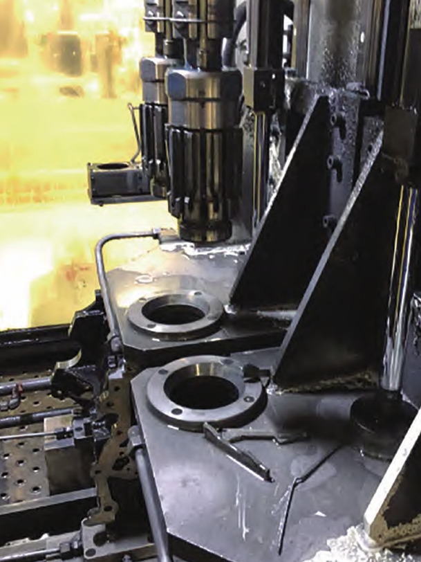
The rapid progress of deep learning has provided a practical path toward intelligent casting defect recognition. Convolutional neural networks can automatically learn discriminative features from images. Unlike hand-crafted features, these learned features can be generalized across multiple defect types and imaging conditions. In this work I propose a complete casting defect recognition framework. The framework includes data-specific augmentation, a deep detection network based on the YOLO paradigm, a custom test-time inference strategy, and a lightweight network optimization. My experiments demonstrate that the proposed method can recognize several common casting defect types with high accuracy and acceptable speed for production-oriented deployment.
Casting Production Background and Defect Mechanisms
I first studied the production process of aerospace light-alloy castings to understand where casting defect can arise. Typical steps include sand mold preparation, melting, pouring, shake-out, grinding, rough machining, nondestructive testing, defect repair, heat treatment, and final inspection. The material goes through complex thermal and mechanical loads. Some casting defects originate from gas solubility changes; others are caused by shrinkage during solidification, inclusion entrapment, or stress-induced crack growth.
In my research, I pay special attention to five major casting defect categories: gas pores, slag inclusions, shrinkage porosity, cracks, and segregation. I summarize their typical formation mechanisms and X-ray appearances in the following table.
| Defect type | Formation mechanism | Radiographic appearance |
|---|---|---|
| Gas pore | Gas dissolved in molten metal or produced by chemical reaction is trapped during solidification | Round or oval dark spot, usually small and sharply outlined |
| Slag inclusion | Foreign particles or nonmetallic materials are mixed into the melt | Irregular bright or dark region, often small, with no fixed shape |
| Shrinkage porosity | Insufficient feeding of liquid metal between dendrites during final solidification | Sponge-like dark patch, often clustered and medium to large in size |
| Crack | Thermal stress or mechanical stress exceeds the strength of the solidifying shell | Thin linear or branched dark indication with sharp ends |
| Segregation | Nonuniform distribution of alloy elements after solidification | Linear or banded region, often lighter than a crack on X-ray image |
These casting defect types differ significantly in shape, size, and contrast. Some defects, such as gas pores and slag inclusions, can be extremely small. Others, such as cracks and shrinkage porosity, may occupy a large area. This diversity poses a strong challenge for manual inspection and for conventional image processing algorithms. In my approach, I avoid designing separate features for each defect type. Instead, I train a deep convolutional network that learns to distinguish all casting defect categories from the data itself.
Data Resources and Image Analysis
The research data used in this study are X-ray images of aerospace light-alloy castings. I obtained the images using an industrial radiography system based on X-ray computed laminography. The equipment produces cross-sectional images of the inspected castings and stores them as digital radiographs. A total of 1451 X-ray images were collected. Among them, 1137 images contain no visible casting defect, while 314 images contain at least one defect. After collaboration with experienced inspectors, I labeled the defects and obtained 421 annotated instances. The labels include five casting defect categories: gas pore, slag inclusion, shrinkage porosity, crack, and segregation.
Each original image has three channels and a spatial resolution of 2176 by 1792 pixels. Manual annotation was performed with the LabelImage tool. The annotation process records the defect type and the bounding box of each casting defect in an XML file. I then used these annotations for supervised training and evaluation. To understand the difficulty of the problem, I analyzed the pixel area of each defect bounding box. I defined defect size using the following rules.
| Size category | Minimum pixel area | Maximum pixel area |
|---|---|---|
| Micro defect | 0 | 6400 |
| Medium defect | 6400 | 40000 |
| Large defect | 40000 | Infinity |
I counted the number of defects in each size category. The results show that micro defects account for about 47 percent of all casting defect instances; large defects also represent a notable fraction; medium-size defects are relatively rare. This imbalance indicates a strong multi-scale property of casting defect targets. At the same time, I computed the aspect ratio of the annotated bounding boxes. Most defects have an aspect ratio smaller than two, but there are also elongated defects with an aspect ratio greater than five. These elongated indications are often cracks or shrinkage bands. Therefore, any robust casting defect recognition model must be able to handle variations in both scale and aspect ratio.
Because the dataset is relatively small, I divided the original data into training and test sets before any augmentation. I used a ratio of 8:2. The training set contains 252 defect images, and the test set contains 62 defect images. All subsequent comparisons use the same split. This split ensures that the test images are not seen during model training and that the reported results reflect the generalization ability of the casting defect detector.
Evaluation Metrics for Casting Defect Detection
In casting defect detection, a predicted bounding box is considered correct when its intersection over union with the ground-truth bounding box is at least 0.5. I use the standard IoU definition
$$IoU = \frac{B_{truth} \cap B_{pred}}{B_{truth} \cup B_{pred}}$$
For each casting defect category, I construct a confusion matrix containing true positive, false negative, false positive, and true negative counts. The precision and recall are defined as
$$Precision = \frac{TP}{TP+FP}$$
$$Recall = \frac{TP}{TP+FN}$$
Precision describes how many predicted casting defect boxes are truly defects. Recall describes how many true casting defect instances are successfully found. In my evaluation, I plot the precision-recall curve by varying the confidence threshold. The average precision for a single defect category is computed as the area under this curve:
$$AP = \int_{0}^{1} p(r) dr$$
The mean average precision over all categories is then
$$mAP = \frac{1}{C} \sum_{i=1}^{C} AP_{i}$$
In addition to precision-oriented metrics, I also pay attention to the miss rate of casting defect detection, which is particularly meaningful for industrial quality control. The leakage or miss rate is defined as
$$LR = 1 – Recall = \frac{FN}{TP+FN}$$
I use mAP as the primary accuracy metric and FPS as the primary speed metric. This combination allows me to evaluate both the quality and the practicality of my casting defect recognition pipeline.
Data Augmentation Adapted to Micro Casting Defects
One of the most important challenges in casting defect recognition is the detection of micro defects. In a deep convolutional detector, repeated down-sampling can reduce a micro defect to only a few pixels in the final feature map. If these features disappear, the casting defect cannot be detected. Moreover, the number of original defect images is far too small to train a deep model without overfitting. I therefore designed a two-stage augmentation strategy: first, overlap cropping; second, Mosaic-based augmentation.
Overlap Cropping
Overlap cropping is inspired by sliding-window detection. I use a fixed window to traverse the original high-resolution X-ray image. The window size is chosen as 300 by 300 pixels, and the stride is selected so that the adjacent windows have an overlap rate of 15 percent. If the window exceeds the image boundary, I shift it backward so that a complete window is always obtained.
When a defect is cut by the window, I need to decide whether the resulting sub-image is useful for learning. I define the retained ratio r as
$$r = \frac{R(B_{gt} \cap B_{sub})}{R(B_{gt})}$$
Here, \(B_{gt}\) is the ground-truth defect bounding box, and \(B_{sub}\) is the sub-image region. The numerator denotes the intersection area between the defect box and the sub-image, while the denominator is the area of the original defect box. When \(r\) is greater than 0.1, I consider the sub-image to contain enough information for training. The selected sub-image is then resized to 448 by 448 pixels.
For large casting defects that are larger than the sliding window, the same defect can appear in several sub-images. This is acceptable because the texture of a large defect remains recognizable after cropping. I also generate an additional training sample by directly resizing the original image to 448 by 448 pixels when the image contains a defect larger than the window. This preserves global context for large casting defect regions.
After overlap cropping, I further enrich the training set with geometric transformations. I use rotations by 90, 180, and 270 degrees, horizontal flipping, and vertical flipping. I also increase the number of transformations for categories with fewer samples. After this stage, the training set is expanded from 252 original high-resolution images to 2779 sub-images with a resolution of 448 by 448 pixels.
Simplified Mosaic Augmentation
Mosaic augmentation is useful because many original X-ray images contain only one casting defect. Training on such sparse images may lead to overfitting and poor generalization. The standard Mosaic method combines four images into one composite image through random cropping and scaling. In my work, I develop a simplified Mosaic strategy that is more suitable for casting defect data.
First, I divide four selected images into four quadrants. Second, I generate a template with width \(w\) and height \(h\). I randomly generate two dividing lines in the horizontal and vertical directions. To avoid very small image regions, each dividing line is constrained to the interval from 0.4 to 0.6 times the corresponding dimension. Third, I split each quadrant using the intersection of these lines. Fourth, I stitch the four split pieces into a new composite image of size \(w \times h\).
In my implementation, I deliberately avoid random color-space transforms. X-ray intensities have a direct physical meaning; changing contrast and brightness may create artificial noise. I also avoid severe random scaling because it can destroy the limited information carried by micro casting defect. Instead, I choose a larger template size of 608 by 608 pixels. This preserves more original information in each quadrant and reduces the chance that a quadrant contains no defect.
During training, I apply the simplified Mosaic augmentation in batches. For each batch containing \(n\) images, I randomly select four images and perform one Mosaic operation. I repeat this process \(n\) times until a new batch of \(n\) images is generated. This procedure is repeated for all batches. The Mosaic operation does not change the total number of images, but it increases the complexity of each image and reduces the imbalance between background and foreground information. More importantly, it makes the detector less likely to overfit to simple single-defect images.
YOLO-Based Casting Defect Detection Network
I choose the YOLO detection paradigm as the basis for my casting defect detection model. YOLO is a one-stage detector that predicts object categories and bounding boxes directly from the input image. Compared with two-stage detectors, YOLO has a simpler pipeline and a much higher inference speed. This is important for real production lines where casting defect inspection must not become a bottleneck.
Core YOLO Concept
The input image is divided into an \(S \times S\) grid of cells. If the center of a real defect falls inside a particular cell, that cell is responsible for predicting that casting defect. Each cell generates several predicted bounding boxes. For each predicted box, the network outputs the center coordinates, width, height, objectness confidence, and class probabilities. The confidence is designed as the product of the probability that an object exists and the IoU between the predicted box and the ground-truth box:
$$C = Pr(obj) \cdot IoU_{pred}^{truth}$$
For each defect category, the final confidence score becomes
$$Score_i = Pr(class_i | obj) \cdot C = Pr(class_i | obj) \cdot Pr(obj) \cdot IoU_{pred}^{truth}$$
During training, the multi-task loss function combines localization loss, confidence loss, and classification loss:
$$L = L_{loc} + L_{conf} + L_{cls}$$
In the early YOLO version, the localization loss treats the center coordinates and width-height dimensions independently. This simple formulation can still work, but it ignores the coupling between these four values. I later improve this by replacing the localization loss with DIoU loss.
Network Architecture
For the feature extraction backbone, I use a Darknet-53 network. Darknet-53 is a residual network that can extract rich features while avoiding gradient degradation. Each convolutional block in Darknet-53 contains a Conv2D layer, a batch normalization layer, and a LeakyReLU activation. The residual block contains two convolutional blocks with kernel sizes 1 by 1 and 3 by 3, and the final output is the sum of the input and the transformed feature.
I use the last three feature maps of the backbone for multi-scale detection. The connection network follows the FPN structure. It performs top-down fusion through up-sampling and concatenation. This design enables the detector to locate casting defect at three different scales. The detection head uses a 3 by 3 convolutional block followed by a 1 by 1 convolution to produce the output tensor. For the input size of 608 by 608 pixels, the three detection heads work on feature maps of size 19 by 19, 38 by 38, and 76 by 76, respectively.
From my analysis, the defect size distribution is highly unbalanced. I therefore use the multi-scale detection strategy to match small defects with high-resolution feature maps and large defects with low-resolution feature maps. This improves the overall recall of casting defect recognition.
Anchor Design Using k-means++
Anchors are prior boxes that help the network predict bounding boxes relative to predefined shapes. In my framework, the anchor size should match the distribution of the actual casting defect bounding boxes. I use k-means++ clustering to design anchors from the training set. The distance between two boxes is based on the IoU metric:
$$d(box_i, box_j) = 1 – IoU(box_i, box_j)$$
In this IoU computation, the two boxes are assumed to have the same center. This distance is more suitable for bounding box clustering than Euclidean distance because it directly reflects shape similarity.
The k-means++ algorithm improves the initialization step. The first initial center is chosen randomly from the data. For every remaining sample, I compute its shortest distance to all existing centers. Then I compute the probability that a sample is selected as the next center:
$$p_{ij} = \frac{D^2(box_i, c_j)}{\sum_{box \in X} D^2(box, c_j)}$$
I use the roulette-wheel method to select the next center according to these probabilities. After the initial centers are determined, the algorithm iteratively assigns each sample to the nearest center and recomputes the center as the mean of all samples in the cluster.
I evaluate different numbers of anchors using the average IoU between all defect boxes and their nearest anchor. The average IoU is defined as
$$AvgIoU = \frac{1}{n} \sum_{i=1}^{n} \max_{j \in [1,k]} IoU(box_i, c_j)$$
The clustering results show that the average IoU increases quickly as the anchor number grows from 1 to 6, but the increase slows down significantly after 6. Therefore, I choose six anchors for my casting defect detection network. The corresponding anchor sizes are listed below.
| Anchor index | Width | Height |
|---|---|---|
| 1 | 55 | 75 |
| 2 | 71 | 155 |
| 3 | 69 | 63 |
| 4 | 94 | 85 |
| 5 | 90 | 83 |
| 6 | 183 | 103 |
These anchors are assigned to the three detection heads according to their scale. Small anchors are assigned to the high-resolution feature map, while large anchors are assigned to the low-resolution feature map.
Test-Time Detection with Bounding Box Suppression
Because my detector is trained on 608 by 608 input images, it cannot process the original 2176 by 1792 test image directly. I therefore apply overlap cropping during inference as well. I use a sliding window of 407 by 407 pixels and then resize each sub-image to 608 by 608 pixels. In addition, I resize the entire original image to 608 by 608 pixels and input this scaled version to the detector. This is necessary to avoid losing large casting defect regions that may span multiple windows.
The final detection result is obtained by mapping the sub-image detections back to their original positions and stitching them together. However, because the sliding windows overlap, the same casting defect can be detected in multiple sub-images. The stitched image may contain many duplicate bounding boxes for one defect. To solve this problem, I propose a bounding-box suppression method.
First, I group all predicted boxes by their predicted category. For each category, I iteratively compute the overlap ratio between two bounding boxes A and B. The two overlap ratios are
$$r_A = \frac{R(A \cap B)}{R(A)}$$
$$r_B = \frac{R(A \cap B)}{R(B)}$$
If either \(r_A\) or \(r_B\) is greater than or equal to a threshold, I keep the box with the smaller value and remove the box with the larger value. In my experiments, a threshold of 0.7 gives good results. If both values are below the threshold, both boxes are retained.
After suppression, I merge remaining boxes that are connected through overlapping relationships. I find groups of boxes in which each box overlaps with at least one other box in the group. Then I replace the whole group with its minimum enclosing rectangle. This final step converts multiple partial predictions into a single bounding box for the same casting defect.
Experimental Results of the Baseline YOLO-Based Method
I trained the baseline YOLO-based casting defect detection network with the following settings. The input size is 608 by 608 pixels. The total number of iterations is 7000. The initial learning rate is 0.002. The learning rate is multiplied by 0.1 at the 2000th and 4000th iterations. I use the pre-trained Darknet-53 weights on the VOC dataset to initialize the backbone. The neck and detection heads are trained from scratch. The test set contains 62 original defect images that are not used in training.
To analyze the contribution of each component, I compare four model combinations. The first model, Model1, uses overlap cropping, Mosaic augmentation, and bounding-box suppression testing. Model2 uses overlap cropping and bounding-box suppression but does not use Mosaic augmentation. Model3 and Model4 do not use overlap cropping. Instead, the original images are directly resized to 608 by 608 pixels. Model3 uses Mosaic augmentation, while Model4 does not.
| Model | Gas pore AP | Slag inclusion AP | Shrinkage porosity AP | Crack AP | Segregation AP | mAP |
|---|---|---|---|---|---|---|
| Model1 | 87.63 | 85.45 | 82.13 | 85.37 | 83.49 | 84.81 |
| Model2 | 84.89 | 83.59 | 81.68 | 84.36 | 82.16 | 83.34 |
| Model3 | 43.11 | 42.81 | 65.84 | 80.21 | 74.26 | 61.25 |
| Model4 | 42.69 | 44.21 | 64.75 | 77.95 | 73.59 | 60.64 |
The comparison shows that overlap cropping significantly improves casting defect detection, especially for gas pores and slag inclusions. These two categories are often micro casting defects. Without overlap cropping, the detector misses many of them. The use of Mosaic augmentation provides a further improvement in mAP. Model1 achieves an mAP of 84.81 percent, which is much higher than the models trained on resized images.
I also compare my method with a traditional sliding-window plus CNN classifier approach. The miss rates for different casting defect categories are shown below.
| Method | Gas pore | Slag inclusion | Shrinkage porosity | Crack | Segregation |
|---|---|---|---|---|---|
| Proposed Model1 | 7.14% | 9.09% | 15.38% | 13.33% | 12.50% |
| SWA + CNN | 17.86% | 18.18% | 23.08% | 20.00% | 12.50% |
The proposed method reduces the miss rate by 7 to 10 percentage points for most defect categories. This validates the effectiveness of the deep learning pipeline. However, the baseline detector is slow. The FPS is only about 0.76 because it processes many overlapping sub-images. I therefore decided to optimize the detection network to improve speed while preserving accuracy.
Lightweight Network Design for Casting Defect Detection
The baseline detector uses many standard 3 by 3 convolutions. The feature extraction backbone Darknet-53 contains more than 50 convolutional layers. This large network produces excellent features, but the computational cost is high. To make casting defect recognition more practical, I introduce depthwise separable convolution as the core operation of the lightweight network.
Depthwise Separable Convolution
A standard convolution operation simultaneously implements spatial filtering and channel fusion. The computational cost of a standard convolution can be written as
$$Cost_{standard} = D_K \cdot D_K \cdot M \cdot N \cdot D_F \cdot D_F$$
Here, \(D_K\) is the kernel size, \(M\) is the number of input channels, \(N\) is the number of output channels, and \(D_F\) is the spatial size of the feature map.
A depthwise separable convolution replaces the standard convolution with two steps. The first step is a depthwise convolution. It applies a single convolutional filter to each input channel. The depthwise convolution cost is
$$Cost_{depthwise} = D_K \cdot D_K \cdot M \cdot D_F \cdot D_F$$
The second step is a pointwise convolution. It uses a 1 by 1 convolution to combine the depthwise output channels. The pointwise cost is
$$Cost_{pointwise} = M \cdot N \cdot D_F \cdot D_F$$
The total cost of a depthwise separable convolution is therefore
$$Cost_{depthwise\_separable} = D_K \cdot D_K \cdot M \cdot D_F \cdot D_F + M \cdot N \cdot D_F \cdot D_F$$
The ratio between the two costs is
$$\frac{Cost_{depthwise\_separable}}{Cost_{standard}} = \frac{1}{N} + \frac{1}{D_K^2}$$
For a typical 3 by 3 convolution with sufficiently large output channel number, the depthwise separable convolution can reduce the computation by roughly 8 to 9 times. In my implementation, I replace all 3 by 3 standard convolutions in the baseline network with depthwise separable convolutional blocks. I keep the 1 by 1 convolutions unchanged because a 1 by 1 pointwise convolution is already efficient.
Inverted Residual Blocks and Improved Attention
Simply replacing standard convolutions with depthwise separable convolutions reduces the number of parameters too much. This can make the model underfit and reduce the casting defect detection accuracy. To overcome this issue, I use inverted residual blocks. In a conventional residual block, the number of channels is first reduced and then expanded. In an inverted residual block, the channel dimension is first expanded and then reduced. This expansion gives the depthwise convolution more channels to work with and increases the feature extraction capacity.
I also incorporate an improved Squeeze-and-Excitation block, abbreviated as SE block. The original SE block performs global average pooling to obtain a channel descriptor. The descriptor is then passed through two fully connected layers. The first fully connected layer uses ReLU, and the second uses Sigmoid. This produces channel weights that are used to rescale the original feature maps.
In my improved SE block, I replace the two fully connected layers with a single one-dimensional convolution. The improved excitation function can be written as
$$s = Sigmoid(C1d(z, \omega))$$
where \(z\) is the channel descriptor after global average pooling, and \(C1d(\cdot)\) denotes a one-dimensional convolution. The kernel size of this one-dimensional convolution is chosen as \(C/16\), where \(C\) is the number of channels. This modification reduces the number of additional parameters while preserving the attention ability of the SE block. The final feature re-calibration is performed as
$$\tilde{X}_c = s_c \cdot X_c$$
where \(X_c\) is the original feature map of channel \(c\), and \(s_c\) is the corresponding channel weight. I combine the improved SE block with the inverted residual block to form a new building unit called SE-DW Residual block. This unit is used as the main block of the lightweight backbone.
Loss Function Improvements
The original YOLO loss function contains three parts. I keep the classification loss, but I improve the localization loss and the confidence loss to address two specific problems.
DIoU Localization Loss
The original localization loss calculates the losses for the center coordinates and the width-height dimensions separately. This means that the four parameters are optimized independently. However, a bounding box is a complete object, and the four parameters should be learned together. I therefore use the Distance-IoU loss, abbreviated as DIoU loss. The DIoU loss is defined as
$$L_{DIoU} = 1 – IoU + \frac{\rho^2(b_{pred}, b_{truth})}{c^2}$$
In this formula, \(b_{pred}\) and \(b_{truth}\) are the centers of the predicted and ground-truth boxes, \(\rho(\cdot)\) is the Euclidean distance, and \(c\) is the diagonal length of the smallest enclosing rectangle. DIoU loss considers both the overlap area and the distance between centers. It makes the regression converge faster and more stably than the original independent regression loss.
Focal Confidence Loss
In casting defect detection, the training image contains many background cells and very few positive cells. This creates a severe imbalance between positive and negative samples. If the model trains mainly on simple negative samples, it may not learn discriminative casting defect features. To solve this problem, I use Focal loss for the confidence loss of negative boxes. The Focal loss is defined as
$$FL = – \alpha_t (1 – \hat{y}_t)^\gamma \log(\hat{y}_t)$$
where \(\alpha_t\) balances the contribution of positive and negative samples, and \(\gamma\) is the focusing parameter that down-weights easy examples. In my experiments, I set \(\alpha_t\) to 0.22 and \(\gamma\) to 2. This helps the network focus more on difficult casting defect examples and reduces the influence of abundant simple background samples.
Results of the Lightweight Casting Defect Detection Network
I retrained the improved model using the same training set, test set, and hyperparameter schedule as the baseline. I use the same bounding-box suppression method for test-time inference. I compare four combinations: the baseline network with the baseline loss, the baseline network with the improved loss, the lightweight network with the baseline loss, and the lightweight network with the improved loss.
| Model | Gas pore AP | Slag inclusion AP | Shrinkage porosity AP | Crack AP | Segregation AP | mAP | FPS |
|---|---|---|---|---|---|---|---|
| Baseline network + baseline loss | 87.63 | 85.45 | 82.13 | 85.37 | 83.49 | 84.81 | 0.76 |
| Baseline network + improved loss | 88.62 | 86.53 | 82.76 | 86.74 | 84.38 | 85.81 | 0.76 |
| Lightweight network + baseline loss | 86.97 | 84.36 | 81.02 | 84.16 | 82.98 | 83.90 | 4.96 |
| Lightweight network + improved loss | 87.84 | 84.68 | 82.24 | 85.51 | 83.96 | 84.85 | 4.96 |
The results show that the improved loss can increase mAP regardless of the network architecture. The lightweight network reduces mAP slightly when combined with the baseline loss, but the gap can be recovered when the improved loss is used. The lightweight network with the improved loss achieves an mAP of 84.85 percent, which is even slightly higher than the original baseline network. At the same time, the inference speed increases from 0.76 FPS to 4.96 FPS. This is about 6.5 times faster and is much more suitable for production line inspection.
I also performed an ablation study to understand the contribution of each improvement. The abbreviations are DW for depthwise separable convolution, G-SE for the improved SE block, DIoU for the DIoU localization loss, and Focal for the Focal confidence loss. The ablation results are shown next.
| DW | G-SE | DIoU | Focal | mAP | FPS |
|---|---|---|---|---|---|
| 84.81 | 0.76 | ||||
| √ | 82.75 | 4.96 | |||
| √ | 85.76 | 0.76 | |||
| √ | 85.52 | 0.76 | |||
| √ | 85.15 | 0.76 | |||
| √ | √ | 83.90 | 4.96 | ||
| √ | √ | √ | 84.07 | 4.96 | |
| √ | √ | √ | √ | 84.85 | 4.96 |
The ablation study reveals several important findings. First, depthwise separable convolution is the main factor that improves the detection speed. Without this change, the FPS remains at 0.76. Second, depthwise separable convolution alone causes a drop in mAP from 84.81 percent to 82.75 percent. This decrease is expected because the network becomes lighter. Third, the improved SE block brings a clear accuracy gain. When used alone, it improves mAP by almost 1 percent. When combined with depthwise separable convolution, it improves mAP by more than 1.3 percent. Fourth, both DIoU loss and Focal loss contribute modest gains. The best accuracy is achieved when all four improvements are used together.
Discussion
My experiments show that the choice of training data representation is critical for casting defect recognition. The overlap cropping strategy directly attacks the micro defect problem. By magnifying local regions, the detector can see small gas pores and slag inclusions as distinct objects instead of losing them in downsampled feature maps. Mosaic augmentation further improves the model’s robustness by increasing the number of defects per image and reducing the risk of overfitting.
The lightweight network design is also essential. The original Darknet-53 backbone is powerful but too heavy for real-time quality control. Depthwise separable convolution is a simple and effective way to reduce computation. The inverted residual structure restores the feature representation capability, while the improved SE block helps the network focus on important channels that encode casting defect information. The improved loss functions stabilize training and improve the final model quality.
There are still some limitations in my work. First, the number of annotated casting defect images is limited. Although augmentation helps, a larger dataset would likely improve accuracy further and reduce the miss rate. Second, the bounding-box suppression method is designed specifically for the sparse distribution of defects in the current dataset. In a denser defect scenario, the merging rule might need to be adjusted. Third, the detection speed of 4.96 FPS is acceptable for offline inspection but may still be insufficient for very high-speed production lines. Further optimization using model pruning, quantization, or TensorRT deployment could be investigated.
Conclusion
In this article, I have presented a deep learning method for casting defect recognition based on X-ray images. I first analyzed the characteristics of aerospace light-alloy casting defect data and identified the challenge of micro defects. I proposed overlap cropping and simplified Mosaic augmentation to adapt the training set to micro defect detection. I then designed a YOLO-based casting defect detection network with multi-scale feature extraction and k-means++ anchor design. To support the overlap-cropped inference pipeline, I proposed a bounding-box suppression method that merges duplicate predictions from overlapping sub-images.
I further optimized the casting defect detection network by introducing depthwise separable convolution, inverted residual blocks, and an improved SE block. I also improved the localization loss with DIoU loss and the confidence loss with Focal loss. The experimental results show that the improved lightweight network achieves an mAP of 84.85 percent and an inference speed of 4.96 FPS, which is about 6.5 times faster than the baseline model. The proposed method reduces the miss rate for most casting defect categories compared with a traditional detection approach.
Future work will focus on expanding the dataset, integrating the model into a complete inspection system, and further compressing the model for real-time edge deployment. I believe that deep learning will continue to play an important role in industrial casting defect recognition and will help manufacturing enterprises improve product quality and production efficiency.