
In the realm of marine engineering, the performance of fluid control systems is paramount, and valves play a critical role in ensuring efficiency and safety. Among these, marine flange globe valves manufactured through steel casting processes are widely utilized in fuel pipeline systems due to their robust construction, reliable sealing, and zero-leakage capabilities. However, the inherent design of straight-through globe valves, where fluid enters from the bottom and exits from the top, often leads to significant flow resistance, reducing overall system efficiency. This high flow resistance coefficient, typically ranging from 4 to 10 depending on nominal size, results in increased energy consumption and diminished flow capacity. In this article, I will delve into an analysis of the flow characteristics of a DN65 marine flange steel casting globe valve, employing numerical simulations and experimental validation to identify key factors affecting performance. Furthermore, I will propose structural optimizations aimed at substantially reducing the flow resistance coefficient and enhancing flow capacity, all while maintaining the valve’s structural integrity. The focus will be on the steel casting aspects of the valve body, as its intricate internal geometry is a primary contributor to flow disturbances. Through this work, I aim to provide insights that can advance the design of steel casting valves for marine applications.
The flow characteristics of valves, particularly flow resistance coefficient (ζ) and flow coefficient (Kv), are vital parameters in pipeline design. These coefficients directly influence the power consumption and flow capacity of the entire system. For steel casting globe valves, the complex internal flow path—comprising an inlet section, a mid-port section, a central cavity, and an outlet section—causes fluid to change direction multiple times, leading to pressure losses and turbulence. To address this, I utilized computational fluid dynamics (CFD) based on the finite volume method (FVM) to simulate the flow field within the valve at a fully open state. The software Flow-Simulation was employed for this purpose, allowing for a detailed finite element analysis of the flow resistance. The geometric model was based on a standard DN65 marine flange steel casting globe valve, with an inlet, mid-port, and outlet diameter of 65 mm, a structural length of 290 mm, and surface roughness of 12.5 μm for the steel casting body. The valve disc, with a planar design and embedded PTFE seal, had a roughness of 6.3 μm and an initial lift of 18.5 mm. To ensure accurate simulation results, extended pipe segments were added—5d at the inlet and 10d at the outlet (where d is the nominal diameter)—to allow for fully developed flow, minimizing boundary effects.
The numerical simulation relied on solving the fundamental governing equations for fluid flow. For incompressible, turbulent flow, the standard k-ε turbulence model was applied, which is well-suited for industrial applications involving steel casting components. The continuity equation and Navier-Stokes (N-S) equations form the basis of the analysis. The continuity equation ensures mass conservation:
$$ \frac{\partial \rho}{\partial t} + \frac{\partial}{\partial x_i} (\rho u_i) = 0 $$
where ρ is the fluid density, t is time, and ui represents the velocity components in the i-direction. The momentum conservation equation, or N-S equation, is expressed as:
$$ \frac{\partial (\rho u_i)}{\partial t} + \text{div} (\rho u_i u) = \text{div} (\mu \cdot \text{grad} u_i) – \frac{\partial p}{\partial x} + S_i $$
Here, μ is the dynamic viscosity, p is the pressure, and Si is the source term. For steady-state analysis, the time-dependent terms are neglected. Additionally, the Bernoulli equation was used to relate pressure and velocity along streamlines:
$$ \frac{p_1}{\rho g} + \frac{v_1^2}{2g} + h_1 = \frac{p_2}{\rho g} + \frac{v_2^2}{2g} + h_2 $$
where p1 and p2 are pressures at two points, v1 and v2 are velocities, h1 and h2 are elevations, and g is gravitational acceleration. The flow resistance coefficient and flow coefficient were calculated from the simulated pressure drops. The flow coefficient Kv is defined as:
$$ K_v = 10 \times Q \times \sqrt{\frac{\rho}{\Delta P_v \times \rho_0}} $$
where Q is the volumetric flow rate (m³/h), ΔPv is the net pressure difference across the valve (kPa), ρ is the fluid density, and ρ0 is the density of water at 15°C. The flow resistance coefficient ζ is given by:
$$ \zeta = \frac{2000 \times \Delta P_v}{\rho \times v^2} $$
with v being the average flow velocity in the pipe (m/s). The mesh generation involved tetrahedral elements for the complex valve regions, with local refinement to capture flow details, resulting in approximately 400,000 cells. Grid independence was verified to ensure solution accuracy. Boundary conditions included inlet flow rates of 42, 48, 54.3, 61.3, and 70 m³/h—covering turbulent flow regimes as per standard requirements—and an outlet pressure of 101.325 kPa. The simulations converged when the inlet total pressure and average velocity stabilized.
The simulation results revealed detailed flow field distributions. For instance, at a flow rate of 70 m³/h, the pressure cloud showed significant pressure gradients within the valve body, with a maximum pressure of 0.192 MPa near the valve disc. Velocity contours indicated high-speed zones in the mid-port section, reaching up to 10.87 m/s, while streamlines displayed vortices and recirculation areas in the inlet and outlet sections, contributing to energy loss. The calculated flow resistance coefficient averaged around 5.29, and the flow coefficient averaged 73.13, consistent with typical values for steel casting globe valves. To validate these findings, experimental tests were conducted in accordance with the GB/T 30832 standard, using a dedicated test bench. The experimental setup included flow meters, pressure transducers, and straight pipe sections to measure the net pressure drop across the valve. The results showed close agreement with simulations, as summarized in Table 1, with discrepancies less than 2.5% for both coefficients, confirming the reliability of the numerical approach.
| Flow Rate (m³/h) | Simulated ΔP (kPa) | Experimental ΔP (kPa) | Simulated ζ | Experimental ζ | Simulated Kv | Experimental Kv |
|---|---|---|---|---|---|---|
| 42.0 | 33.38 | 31.78 | 5.33 | 5.34 | 72.70 | 73.09 |
| 48.0 | 43.53 | 44.03 | 5.32 | 5.34 | 72.75 | 73.10 |
| 54.3 | 55.62 | 54.11 | 5.31 | 5.34 | 72.81 | 73.14 |
| 61.3 | 69.65 | 70.28 | 5.22 | 5.34 | 73.45 | 73.12 |
| 70.0 | 91.61 | 96.71 | 5.27 | 5.32 | 73.14 | 73.22 |
Analyzing the flow field, it became evident that the steel casting valve body’s internal geometry was the primary factor causing high flow resistance. The inlet section transitioned from a circular to a U-shaped cross-section, creating sharp turns and stagnant zones. The mid-port section had a small area with abrupt directional changes, while the central cavity was constrained, and the outlet section featured discontinuities that induced vortices. To address these issues, I proposed an optimized design focusing on streamlining the flow path without altering the overall structural length—a key consideration in steel casting manufacturing to maintain compatibility with existing pipelines. The optimization principles included: increasing the inlet and outlet diameters from 65 mm to 67 mm (maximum limit per tolerance standards) to expand the flow area; reshaping the inlet section with smooth, rounded transitions to reduce flow separation; enlarging the mid-port diameter to 73 mm with fillet edges to minimize secondary flow angles; expanding the central cavity cross-sectional area to approximately three times the inlet area; increasing the valve disc lift to one-third of the nominal diameter (22 mm) to reduce obstruction; and contouring the outlet section for gradual contraction. These modifications aimed to reduce pressure losses and turbulence, leveraging the flexibility of steel casting processes to achieve complex geometries.
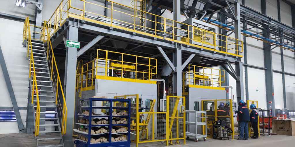
The steel casting process is instrumental in producing such optimized valve bodies, as it allows for precise control over internal shapes and surface finishes, which are crucial for flow performance. After implementing these changes, I performed another round of CFD simulations under identical boundary conditions. The results demonstrated marked improvements: the maximum pressure dropped by 26.3% to 0.14 MPa, and the peak velocity decreased by 11.5% to 9.63 m/s. Streamlines became smoother, with reduced vortices and more uniform flow distribution. The calculated flow resistance coefficient averaged 2.81, and the flow coefficient averaged 105.99, indicating a substantial enhancement. To verify this, a prototype of the optimized steel casting valve was manufactured and tested on the same experimental bench. The data, presented in Table 2, showed excellent correlation with simulations, with flow resistance coefficient errors below 5% and flow coefficients consistently above 102, underscoring the success of the optimization.
| Flow Rate (m³/h) | Simulated ΔP (kPa) | Experimental ΔP (kPa) | Simulated ζ | Experimental ζ | Simulated Kv | Experimental Kv |
|---|---|---|---|---|---|---|
| 42.0 | 15.83 | 16.52 | 2.84 | 2.73 | 105.58 | 102.21 |
| 48.0 | 20.58 | 22.62 | 2.83 | 2.69 | 105.81 | 102.89 |
| 55.0 | 26.90 | 27.81 | 2.82 | 2.70 | 106.05 | 102.68 |
| 63.0 | 35.14 | 36.04 | 2.80 | 2.74 | 106.28 | 102.09 |
| 72.0 | 45.71 | 45.94 | 2.75 | 2.69 | 106.50 | 102.96 |
To further quantify the relationship between the steel casting valve body’s geometry and flow resistance, I derived formulas linking the curvature of the inlet section to the flow resistance coefficient. For the front part of the inlet, the curvature K1 relates to the nominal diameter d by:
$$ d \approx \frac{10}{7 \cdot K_1} $$
Substituting into the flow resistance equation yields:
$$ \zeta \approx \frac{5140 \times \Delta P_v}{\rho \times K_1^4 \times Q^2} $$
For the rear part of the inlet, with curvature K2:
$$ d \approx \frac{10}{13 \cdot K_2} $$
and thus:
$$ \zeta \approx \frac{432 \times \Delta P_v}{\rho \times K_2^4 \times Q^2} $$
These expressions highlight how subtle changes in steel casting design, such as curvature adjustments, can significantly impact flow performance. In practice, the optimized valve achieved a 49.3% reduction in average flow resistance coefficient (from 5.34 to 2.71) and a 40.2% increase in average flow coefficient (from 73.13 to 102.55). This improvement translates to lower energy losses and higher flow capacity in marine systems, making steel casting valves more efficient. The optimization also considered manufacturing constraints; for instance, the enlarged flow areas and rounded corners are feasible through advanced steel casting techniques, which ensure dimensional accuracy and surface quality. Moreover, the increased valve disc lift enhances operational flexibility without compromising sealing, a critical aspect for steel casting globe valves in demanding environments.
In conclusion, this study demonstrates the effectiveness of combining numerical simulation and experimental validation to optimize the flow characteristics of marine flange steel casting globe valves. By focusing on the internal geometry of the steel casting valve body, I identified key areas for improvement, such as the inlet, mid-port, and outlet sections, and implemented design changes that drastically reduced flow resistance and increased flow capacity. The optimized steel casting valve not only performs better but also aligns with industry standards for structural length and compatibility. These findings underscore the importance of meticulous design in steel casting processes for fluid control components, offering a roadmap for future developments in valve engineering. As marine systems evolve towards greater efficiency, such optimizations in steel casting technology will play a pivotal role in enhancing performance and sustainability.