Online Inspection for 3D Sand Printing Using Machine Vision

In this article, I present my research work on developing an online inspection system for 3D sand printing based on machine vision. The core contribution is a set of algorithms for precise image segmentation, dimensional accuracy prediction, and defect recognition, all integrated into a practical detection device for sand mold manufacturing. I first introduce the background and motivation, then describe the system design, followed by the improved Markov Random Field segmentation method, the sand mold accuracy estimation technique, and finally the YOLOv5‑based defect detection approach. My experimental results demonstrate that the proposed methods achieve high accuracy and reliability, providing a viable solution for real‑time quality control in 3D sand printing.

1. Introduction

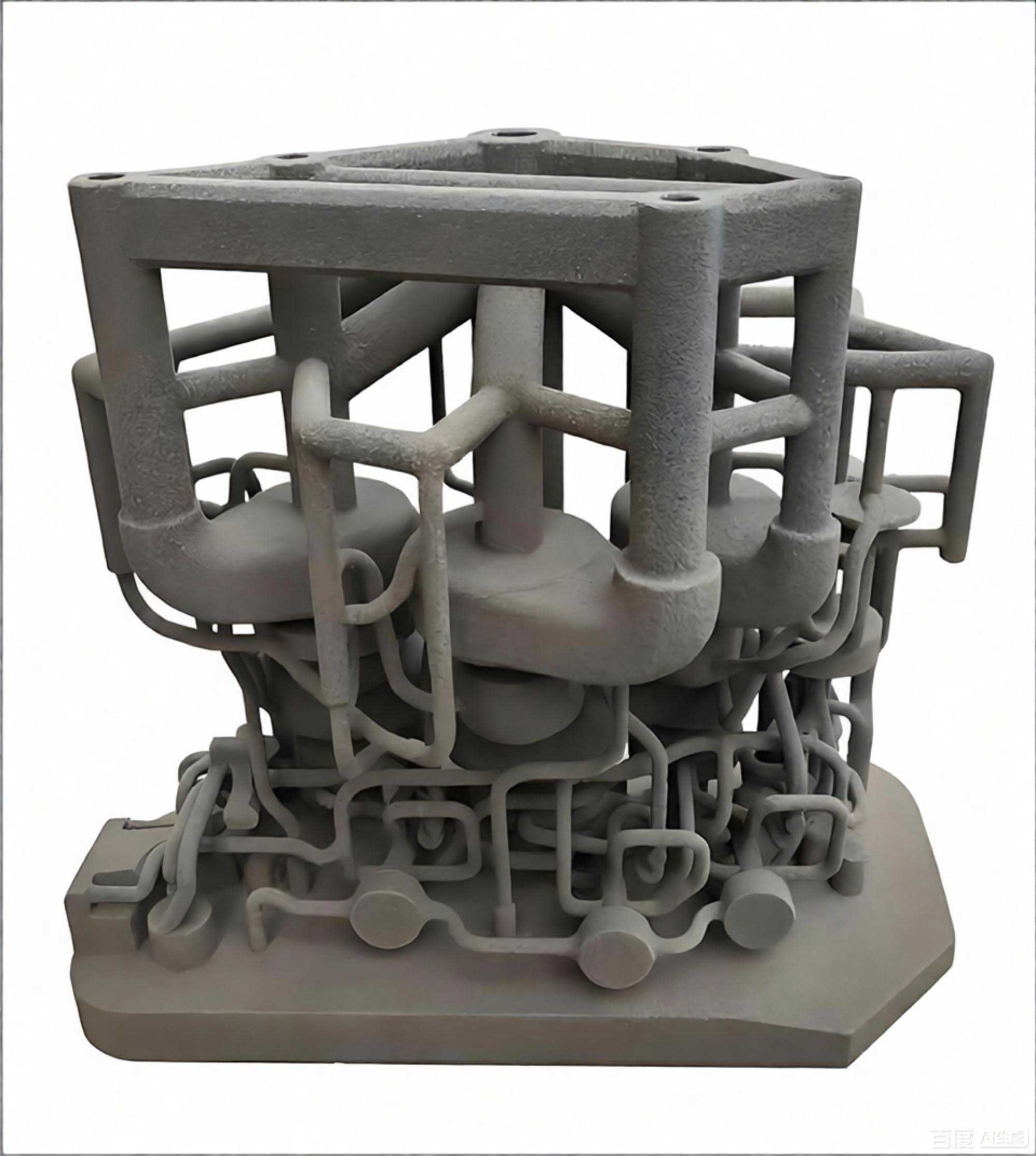
Sand mold 3D printing, also known as inkjet sand printing, is an additive manufacturing process that creates sand molds layer by layer. Compared with traditional sand casting, this technology offers significant advantages in producing complex sand molds, reducing research and development time, and lowering costs for single and small batch production. The quality of the sand mold directly determines the quality of the final casting. Among the many quality attributes, dimensional accuracy and surface defects are the most critical factors. However, in current practice, inspection is usually performed after printing, using manual tools such as calipers and gauges. This approach is time‑consuming, inconsistent, and often damages the fragile sand mold surface.

To overcome these limitations, I developed a machine vision‑based online inspection system capable of measuring the size and detecting typical defects during the 3D sand printing process. My work covers the following aspects:

• Design and integration of a vision system on a sand mold 3D printer, including camera, lens, light source, and mechanical structure.
• An improved Markov Random Field (MRF) image segmentation algorithm adapted to the noisy and blurred edges of sand mold images.
• A dimensional accuracy prediction method based on the analysis of multiple printed layers, using fitted circle centers to estimate the overall size error.
• A defect recognition method based on the YOLOv5 convolutional neural network for typical defects such as insufficient sand coverage and scratches.

I began by reviewing the state of the art in image segmentation, machine vision inspection, and object detection. The literature shows that MRF models have been successfully applied to medical images with similar characteristics (weak boundaries, high noise, and low signal‑to‑noise ratio), but rarely to sand mold images. Likewise, YOLOv5 has become a popular framework for real‑time defect detection in industrial applications, yet its use in sand printing is still limited. My research aims to fill this gap by tailoring these algorithms to the specific needs of sand mold 3D printing.

2. Development of the Online Inspection System

2.1 System Architecture

The online inspection system is mounted on a commercial sand mold 3D printer. The printer uses a moving hopper and scraper to spread a layer of sand mixed with a curing agent, followed by an inkjet printhead that selectively deposits a furan resin. The inspected sand mold images are acquired after each printing layer (or after a few layers) without interrupting the printing cycle. The vision system is placed above the sand tank, ensuring an unobstructed view of the entire build area. Figure 1 shows the overall hardware arrangement.

2.2 Hardware Selection

The inspection area is 600 mm × 500 mm. Based on the required measurement accuracy of ±0.15 mm, I calculated the minimum number of pixels needed in each direction:

$$ N_x = \frac{600\ \text{mm}}{0.6\ \text{mm}} \times 1000 = 1000 \ \text{pixels} $$
$$ N_y = \frac{500\ \text{mm}}{0.6\ \text{mm}} \times 1000 = 834 \ \text{pixels} $$

To obtain better edge definition, I chose a higher‑resolution camera: the Hikvision MV‑CE200‑10GM, a 20‑megapixel industrial area scan camera with a resolution of 5472 × 3648 pixels. Table 1 summarizes its key parameters.

Table 1: Camera specifications

Parameter	Value
Sensor	20 MP CMOS
Resolution	5472 × 3648
Frame rate	5.9 fps
Signal-to-noise ratio	41.5 dB
Dynamic range	65.5 dB

The working distance from the lens to the sand surface is about 1145 mm. The required focal length was computed with the lens equation:

$$ f = \frac{WD \times \text{size}}{fov} = \frac{1145 \times 2.4 \times 10^{-3}}{600} \times 5472 \approx 25.17\ \text{mm} $$

Therefore, I selected a Hikvision MVL‑KF2528M‑12MP lens with a 25 mm focal length, a maximum field of view of 674 mm × 521 mm, and an optical distortion of only 0.40%. Its parameters are given in Table 2.

Table 2: Lens specifications

Parameter	Value
Focal length	25 mm
Optical distortion	0.40%
Field of view	36.7°
Aperture range	F2.8 – F16

For illumination, I used a high‑angle ring light (Hikvision MV‑LRSS‑H‑80‑W) that provides uniform lighting over the entire build area without causing glaring reflections. The ring light is mounted around the camera lens, and its angle can be adjusted to enhance the contrast between the printed pattern and the sand background.

2.3 Mechanical Structure

To stabilize the optics, I designed a lightweight aluminum frame that suspends the camera, lens, and light source above the center of the sand tank. The frame is vibration‑damped and allows precise vertical adjustment of the camera height. The hardware was installed without interfering with the motion of the inkjet carriage or the sand spreading system. This non‑invasive installation ensures that the inspection does not disturb the printing cycle.

2.4 Image Characteristics of Sand Molds

Sand mold images have several unique properties that complicate automated processing:

• High noise level: The sand surface consists of individual grains with different shapes and orientations, producing a texture that resembles Gaussian noise. This noise often overwhelms the true edges.
• Weak boundaries: The resin is sprayed as a fine mist and then penetrates into the sand, creating a gradual transition zone at the boundary of the printed pattern. As a result, the edge is not a sharp line but a soft gradient, making exact localization difficult.
• Large data volume: A single 5472 × 3648 color image contains more than 50 million bytes of data. Processing such large images in real time requires efficient algorithms.

Figure 2 illustrates a typical sand mold image and its threshold‑segmented version, showing how the threshold operation dramatically degrades the edge quality.

2.5 Typical Defects in Sand Mold Printing

During the printing process, two common defects often appear: sand surface scratches and insufficient sand coverage. Scratches are usually caused by large sand particles or foreign objects that are dragged across the surface by the scraper. Insufficient coverage occurs when the amount of sand supplied is lower than required, creating voids or thin areas that can cause layer delamination or dimensional errors in the final mold. Representative defect images are shown in Figure 3.

3. Improved Sand Mold Image Segmentation Algorithm

3.1 Why MRF?

Classical edge detection methods (Sobel, Canny, etc.) and clustering algorithms (thresholding, k‑means, SLIC) often fail on sand mold images because the edges are too blurred and the noise is too strong. After testing several approaches, I found that Markov Random Field (MRF) modeling is particularly suitable for this type of image. MRF treats pixel labels as random variables with spatial dependencies, allowing the model to enforce local consistency and overcome noise. I first implemented a standard MRF with Iterated Conditional Modes (ICM) and observed that the segmentation still had jagged edges and small artificial protrusions, as shown in Figure 4.

3.2 Background of MRF

Define the set of all pixel coordinates $S$ in an $M \times N$ image. Each pixel $s \in S$ has an observed gray value $y_s$. The goal is to assign a class label $x_s$ from a set $\Lambda = \{1, 2, \ldots, L\}$. According to Bayesian theory, the maximum a posteriori (MAP) estimate is obtained by maximizing the posterior probability:

$$ P(X \mid Y) \propto P(Y \mid X) P(X) $$

The likelihood $P(Y \mid X)$ is usually assumed to be Gaussian for each class. Under the MRF model, the prior $P(X)$ follows a Gibbs distribution:

$$ P(X) = \frac{1}{Z} \exp\left( -U(X) \right), \quad U(X) = \sum_{c \in C} V_c(X) $$

where $U(X)$ is the energy function, $V_c$ is the potential function defined on cliques $c$, and $C$ is the set of all cliques in the neighborhood system. The ICM algorithm iteratively updates each label to minimize the local energy, thereby approximating the MAP solution.

3.3 Proposed Modification

To suppress the jagged artifacts, I incorporated an additional potential term into the energy function. The new potential function $V_s$ for a central pixel $s$ with a second‑order neighborhood is:

$$ V_s = \begin{cases}
\beta & \text{if } N_{i,j} \ne N_{i-1,j} \ne N_{i+1,j} \text{ or } N_{i,j} \ne N_{i,j-1} \ne N_{i,j+1}\\
\beta & \text{if } N_{i,j} \ne N_{i-1,j-1} \ne N_{i+1,j+1} \text{ or } N_{i,j} \ne N_{i-1,j+1} \ne N_{i+1,j-1}\\
-\beta & \text{otherwise}
\end{cases} $$

Here, $N_{i,j}$ is the label of the pixel at $(i,j)$. This function assigns a higher penalty to configurations that create thin one‑pixel protrusions (jagged edges), thus discouraging them. The total energy becomes:

$$ U_{\text{total}} = U_{\text{likelihood}} + U_{\text{prior}} + \sum_{s} V_s $$

The ICM algorithm is then run to minimize this modified energy function.

3.4 Experiments and Results

I compared my improved MRF algorithm with threshold segmentation and the standard MRF‑ICM method. The test image was captured 10 seconds after printing a layer to balance image quality and process speed. For quantitative evaluation, I used the intersection‑over‑union (IoU), pixel accuracy (PA), and class pixel accuracy (CPA). Because the interior of the printed pattern is nearly the same across all three methods, I focused on the edge region (see Figure 5). The ideal edge was delineated by the computer‑aided design (CAD) model projected onto the image.

Table 3: Performance comparison of segmentation methods

Method	Edge IoU	Edge PA	Edge CPA
Threshold	0.528	0.806	0.813
Standard MRF	0.579	0.854	0.872
Improved MRF	0.618	0.881	0.912

As shown in Table 3, my improved MRF raises the edge IoU by 17.05% over threshold segmentation, the edge PA by 9.31%, and the edge CPA by 12.18%. Although the absolute improvement over the standard MRF is modest, it significantly reduces the number of jagged pixels, yielding a much cleaner contour that is crucial for accurate dimensional measurement.

4. Sand Mold Dimensional Accuracy Prediction

4.1 Motivation and Principle

In sand 3D printing, the resin diffuses into the sand, leading to an effective expansion of the printed area compared to the ideal CAD model. This expansion varies from layer to layer due to printing parameters, environmental conditions, and machine motion errors. Instead of measuring the final dimensions after printing, I proposed an online method that estimates the accuracy from the image of each printed layer. I used a special test specimen called an “eight‑character block” (or “8‑block”), whose contour consists of six circular arcs with different radii. By fitting circles to these arcs, I obtained the positions of six circle centers. The variation of these center positions across multiple layers correlates with the overall dimensional error of the printed part.

4.2 Processing Pipeline

The online accuracy estimation follows these steps:

1. Image acquisition: Capture an image of the printed surface after a fixed waiting period.
2. Distortion correction: Correct the lens distortion using a calibrated camera model.
3. Region of interest (ROI): Locate the eight‑character block in the image using the known printing coordinates.
4. Segmentation: Apply the improved MRF algorithm to separate the printed pattern from the sand background.
5. Feature extraction: Extract the contours and fit circles to the six arcs using the least‑squares method.
6. Error analysis: For each arc, compute the standard deviation of the fitted circle center across multiple printing layers.

The circle fitting was performed using the least‑squares method, which minimizes the sum of the squared distances from the observed contour points $(x_i, y_i)$ to the fitted circle:

$$ \min_{a,b,r} \sum_{i=1}^{m} \left( \sqrt{(x_i – a)^2 + (y_i – b)^2} – r \right)^2 $$

where $(a, b)$ is the circle center and $r$ is the radius. The estimated center positions are then analyzed layer by layer.

4.3 Experimental Validation

I printed an eight‑character block with a wall thickness of 10 mm. Every 1 mm of printing (two layers), I captured an image and applied the segmentation and circle‑fitting pipeline. Table 4 lists the fitted circle centers for one arc over ten repeated measurements (in pixel coordinates).

Table 4: Fitted circle center positions for one arc over ten measurements

Measurement	X (pixel)	Y (pixel)
1	321.41	204.57
2	315.57	197.82
3	321.41	204.57
4	321.41	204.78
5	321.34	204.82
6	321.58	204.21
7	321.75	204.52
8	321.82	204.62
9	321.91	204.49
10	320.99	204.17

From these coordinates, I computed the standard deviation in X and Y:

$$ S_x = \sqrt{ \frac{1}{n-1} \sum_{i=1}^{n} (x_i – \bar{x})^2 } = 0.2688 $$
$$ S_y = \sqrt{ \frac{1}{n-1} \sum_{i=1}^{n} (y_i – \bar{y})^2 } = 0.2092 $$

The total center fluctuation for this arc is then $F = \sqrt{S_x^2 + S_y^2}$ (converted to millimeters using the pixel‑to‑millimeter scale factor). Similar fluctuations were computed for all six arcs in each layer. The mean fluctuation of the six centers was used as a single metric for the entire layer.

I repeated the experiment for eight different printed specimens, each with a slightly different printing condition. For each specimen, I recorded the mean center fluctuation and the actual dimensional error of the final block (measured with a coordinate measuring machine). The data are given in Table 5.

Table 5: Center fluctuation and actual dimensional error for eight specimens

Specimen	Mean Fluctuation (mm)	Actual Dimensional Error (mm)
1	3.682 × 10⁻⁴	0.724
2	5.908 × 10⁻⁴	0.881
3	6.108 × 10⁻⁴	0.916
4	3.190 × 10⁻⁴	0.710
5	4.653 × 10⁻⁴	0.865
6	3.393 × 10⁻⁴	0.704
7	3.592 × 10⁻⁴	0.693
8	4.360 × 10⁻⁴	0.825

The Pearson correlation coefficient between the mean fluctuation and the actual error is:

$$ \rho = \frac{ \sum_{i=1}^{n} (F_i – \bar{F})(E_i – \bar{E}) }{ \sqrt{ \sum_{i=1}^{n} (F_i – \bar{F})^2 } \sqrt{ \sum_{i=1}^{n} (E_i – \bar{E})^2 } } = 0.941 $$

This high positive correlation confirms that the center fluctuation can be used as a reliable predictor of the dimensional error. A linear regression yields:

$$ E = 1748 \times F $$

where $E$ is the predicted dimensional error and $F$ is the mean center fluctuation. With this model, the prediction error of the method is within ±0.15 mm, which satisfies the accuracy requirement of the sand printing process. The prediction can be performed online after every few layers, allowing early detection of abnormal deviations and enabling corrective actions such as adjusting resin dosage or recalibrating the printhead.

5. Defect Recognition Based on Convolutional Neural Networks

5.1 Why YOLOv5?

Traditional image processing methods for defect detection rely on hand‑crafted features and are often specific to a single defect type. In sand 3D printing, defects can vary in shape, size, and intensity, making it difficult to design a universal algorithm. Convolutional neural networks (CNNs) have shown outstanding performance in object detection and classification. Among the many CNN‑based detectors, YOLOv5 provides an excellent trade‑off between speed and accuracy, making it suitable for real‑time online inspection.

5.2 Network Architecture and Improvements

The YOLOv5 framework consists of an input end, a backbone, a neck, and a prediction head. The key improvements over previous YOLO versions include:

• Mosaic data augmentation: Four training images are randomly scaled, cropped, and stitched together to create a new sample, thereby increasing the variety of object scales and backgrounds and reducing overfitting.
• Focus layer: This layer slices the input image into four sub‑images and stacks them along the channel dimension, effectively increasing the receptive field without losing information.
• SPP module: Spatial Pyramid Pooling captures multi‑scale features by applying max‑pooling with different kernel sizes, improving the detection of objects of varying sizes.
• PANet neck: Path Aggregation Network enhances the flow of information from lower layers to higher layers, enabling better detection of small objects.

5.3 Dataset and Experimental Setup

I collected 2176 images of 5472 × 3648 pixels from the sand printing process. After cropping to regions of interest and manual filtering, I selected 1562 defect images, with 1249 for training and 313 for testing. The defects were labeled into two categories: “01” for insufficient sand coverage and “02” for sand surface scratches. Each image contained either one or both defects, and some images also contained a printed pattern, making the detection more challenging. Data augmentation (Mosaic) was applied during training to increase robustness.

The experiments were carried out on a computer with an Intel Core i5‑8400 CPU, 8 GB RAM, and Windows 10. I used PyCharm with PyTorch as the deep learning framework. The training parameters are listed in Table 6.

Table 6: Training parameters for YOLOv5

Parameter	Value
Image size	640 × 640
Confidence threshold	0.25
IoU threshold	0.45
Epochs	50
Batch size	16
Optimizer	SGD
Pretrained weights	YOLOv5s.pt

5.4 Evaluation Metrics

The detection performance was evaluated using precision (P), recall (R), mean average precision (mAP), and the average mAP over IoU thresholds from 0.5 to 0.95. These metrics are defined as:

$$ P = \frac{TP}{TP + FP}, \quad R = \frac{TP}{TP + FN} $$
$$ AP = \sum_{i=1}^{n} (r_i – r_{i-1}) p(r_i) $$
$$ mAP = \frac{1}{K} \sum_{k=1}^{K} AP_k $$

where TP, FP, FN denote true positives, false positives, and false negatives, respectively. The mAP@0.5 corresponds to the mAP at an IoU threshold of 0.5, while mAP@0.5:0.95 is the average over thresholds 0.5, 0.55, …, 0.95.

5.5 Results and Discussion

After 50 epochs, the training showed good convergence. The final evaluation metrics are given in Table 7.

Table 7: Detection results on the test set

Class	Images	Labels	P	R	mAP@0.5	mAP@0.5:0.95
All	591	953	0.864	0.907	0.922	0.723
01 (insufficient sand)	591	576	0.877	0.967	0.974	0.770
02 (scratch)	591	377	0.852	0.846	0.869	0.680

The model achieved an overall precision of 86.4% and a recall of 90.7%, with an mAP@0.5 of 0.922. The insufficient sand defect was detected with particularly high recall (96.7%), while the scratch defect had a lower but acceptable recall (84.6%). The loss curves (classification loss, localization loss, and confidence loss) all decreased steadily, indicating stable training. Figure 6 shows an example of the detection output on a test image containing both defect types.

These results demonstrate that the YOLOv5‑based approach can effectively recognize the typical defects encountered in sand 3D printing. The relatively high recall means that most actual defects are caught, which is crucial for quality control. The precision indicates a low rate of false positives, which is also desirable to avoid unnecessary interventions.

6. Conclusion and Future Work

In this work, I developed a complete machine‑vision‑based online inspection system for 3D sand printing. The system includes carefully selected hardware components and a set of advanced image‑processing algorithms. My main contributions are summarized as follows:

1. I designed and integrated a vision system on a sand mold 3D printer, achieving high‑quality image acquisition without interfering with the printing process.
2. I proposed an improved Markov Random Field segmentation algorithm that effectively handles the noisy and blurred edges of sand mold images, increasing the edge IoU by 17% over thresholding and reducing jagged artifacts.
3. I introduced a novel method for dimensional accuracy prediction based on the statistical fluctuation of fitted circle centers from printed arcs. The method shows a strong correlation (0.941) with actual size errors and achieves a prediction accuracy of ±0.15 mm, enabling online process monitoring and early corrective actions.
4. I applied the YOLOv5 convolutional neural network for defect detection, achieving an overall precision of 86.4%, recall of 90.7%, and mAP@0.5 of 0.922 for the two most common defect types in sand printing: insufficient sand coverage and surface scratches.

These algorithms are not limited to sand 3D printing; they can also be adapted to other industrial inspection tasks involving weak edges, high noise, and multi‑scale defects. In future work, I plan to extend the defect dataset to include additional defect classes and background images to further improve the model’s generalization. I also intend to optimise the computational efficiency of the segmentation and detection algorithms so that they can run on embedded hardware with lower latency. Furthermore, I will explore the use of unsupervised or few‑shot learning to reduce the dependency on large annotated datasets. Ultimately, the goal is to realize a fully autonomous, closed‑loop quality control system for sand 3D printing, where any deviation from the desired quality automatically triggers process adjustments, thereby maximizing yield and minimizing waste in an industrial setting.