
In my research, I focus on developing an automated visual inspection system for sand foundry defects. The work is motivated by the fact that castings produced in sand foundries often exhibit surface flaws such as dark holes, shallow pits, cracks, bulges, depressions, and notches. These sand foundry defect types not only degrade the structural integrity of the component but also create potential safety hazards when the parts are assembled into larger systems. Traditional inspection methods, which rely on human eyes or simple physical sensors, are either too slow, too expensive, or too inconsistent for modern industrial production lines. As a result, I propose a deep learning based approach that can automatically identify and classify sand foundry defect instances with high accuracy and speed.
The main difficulty in applying deep learning to sand foundry defect detection is the need to preserve fine visual details while processing large images. In my setup, I use a 5-megapixel industrial camera that captures images of size 2566×1940 pixels. These high-resolution images are necessary because many sand foundry defect features are only a few pixels in size, such as a dark hole that may occupy only 10×10 pixels. If I naively resize the entire image to the typical 256×256 input size used by most convolutional neural networks, the defect information is lost. Another challenge is the high variability of the casting surface texture. Since the surface is usually sandblasted or machined, it naturally contains spots, tiny scratches, and uneven regions that are not defects. These background patterns create strong interference and can easily fool a classifier. Furthermore, different classes of sand foundry defect often share similar visual characteristics. For instance, a dark hole and a shallow pit both appear as dark circular regions, and the only reliable difference lies in their depth and size. The inter-class similarity and intra-class variance make the classification task particularly difficult.
Overall Algorithm Architecture
To overcome the problems of small targets and high resolution requirements, I designed a two-stage algorithm. Instead of directly searching for defects in the full-size image, the algorithm first localizes the regions of interest on the casting. The underlying idea is to transform the original task of “finding tiny targets from a huge image” into two simpler tasks: first, find medium-sized casting regions from the huge image; second, detect tiny defects from these medium-sized regions. This approach preserves the defect details because the medium-sized regions are cropped from the original 2566×1940 image and only resized to 256×256 after cropping. The resizing operation does not dramatically reduce the information content of a region that originally spans 200×200 to 500×500 pixels.
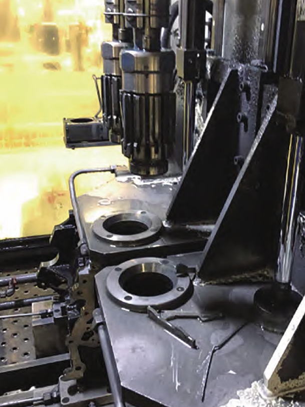
Figure 1 shows a typical engine cylinder block that I use as an example of a sand foundry product. The casting in my experiments is an automobile brake bracket, which has a U-shape body with several flat surfaces and corner areas. The regions that most frequently contain defects are the top-left platform, top-left link, bottom-left link, top-right platform, top-right link, and bottom-right link. I train a YOLO (You Only Look Once) network to detect these six regions from the input image. Once the regions are located, the algorithm crops them from the original high-resolution image and resizes each crop to 256×256 pixels. Then a second network, based on the ResNet-50 architecture with my modifications, classifies each region into one of seven categories: no defect, dark hole, shallow pit, crack, bulge, depression, or notch.
The flow of the complete system is as follows. First, the original 2566×1940 image is sent to a preprocessing module that removes known background regions and then resizes the remaining area to 416×416. The resized image is passed through the YOLO network. If no casting region is found, the image is marked as an invalid sample. If at least one region is detected, the predicted bounding boxes are mapped back to the original image coordinates, and the corresponding regions are cropped. Every cropped region is then resized to 256×256 and passed through the improved ResNet-50 classifier. The classifier outputs a probability distribution over the seven classes. If the predicted class is one of the six defect types, the system records that a sand foundry defect is present and outputs its category along with the location of the region in the original image. If all regions are classified as “no defect”, the system marks the entire casting as defect-free.
Region Detection with YOLO-v3
For the first stage, I use the YOLO-v3 architecture, which treats object detection as a regression problem. The network takes a 416×416 input and divides the image into an S×S grid. Each grid cell is responsible for predicting bounding boxes and confidence scores for objects whose centers fall inside the cell. The YOLO-v3 model uses Darknet-53 as its backbone, which is composed of 53 convolutional layers with residual connections. The network outputs feature maps at three different scales, enabling the detection of objects of varying sizes. Since the casting regions are relatively large and have stable geometric shapes, YOLO-v3 performs well for this localization task.
In my experiments, I use the same data preparation procedure as commonly used in object detection. The original images are annotated with bounding boxes for the six casting regions. Each bounding box is defined by its center coordinates \((x, y)\), its width \(w\), its height \(h\), and a class label \(c\). The loss function of YOLO-v3 is a sum of three components: the bounding box coordinate loss, the confidence loss, and the classification loss. The coordinate loss is computed using the sum of squared errors, but only for boxes that are responsible for a ground-truth object. The confidence loss is a binary cross-entropy term that penalizes incorrect objectness predictions. The classification loss is also a binary cross-entropy term, but it is only applied when an object is present. The overall loss function can be expressed as:
$$\mathcal{L}_{YOLO} = \lambda_{coord} \sum_{i=0}^{S^2} \sum_{j=0}^{B} \mathbb{1}_{ij}^{obj} \left[ (x_i – \hat{x}_i)^2 + (y_i – \hat{y}_i)^2 \right] + \lambda_{coord} \sum_{i=0}^{S^2} \sum_{j=0}^{B} \mathbb{1}_{ij}^{obj} \left[ (\sqrt{w_i} – \sqrt{\hat{w}_i})^2 + (\sqrt{h_i} – \sqrt{\hat{h}_i})^2 \right] + \sum_{i=0}^{S^2} \sum_{j=0}^{B} \mathbb{1}_{ij}^{obj} C_{ij} \log(\hat{C}_{ij}) + \lambda_{noobj} \sum_{i=0}^{S^2} \sum_{j=0}^{B} \mathbb{1}_{ij}^{noobj} C_{ij} \log(\hat{C}_{ij}) + \sum_{i=0}^{S^2} \mathbb{1}_{i}^{obj} \sum_{c \in classes} [\hat{p}_i(c) \log(p_i(c)) + (1 – \hat{p}_i(c)) \log(1 – p_i(c))]$$
where \(\mathbb{1}_{ij}^{obj}\) indicates whether the \(j\)-th bounding box in cell \(i\) is responsible for detecting an object, \(\mathbb{1}_{ij}^{noobj}\) indicates the opposite, \(\lambda_{coord}\) and \(\lambda_{noobj}\) are weighting factors, and the hat symbols denote predicted values. The square-root terms for width and height are used to reflect the fact that small deviations in large boxes matter less than small deviations in small boxes.
Dataset and Training for YOLO
I collected 850 physical samples of the brake bracket. From these, I selected 625 images as the raw dataset. To increase the amount of data and improve the robustness of the network, I performed data augmentation by applying random translations, rotations, and scaling. Each image was expanded to four different versions, resulting in a total of 2500 images. Two thousand images were used for training and 500 for testing. The training process ran for 100 epochs, with a batch size of 10 images. Table 1 shows the accuracy, intersection-over-union (IoU), and frames per second (FPS) values at selected epochs during training.
| Epoch | Training Accuracy | Test Accuracy | IoU Score | FPS |
|---|---|---|---|---|
| 5 | 38.5% | 33.4% | 0.45 | 34 |
| 10 | 66.3% | 61.3% | 0.53 | 34 |
| 15 | 75.2% | 67.2% | 0.67 | 34 |
| 20 | 80.8% | 74.2% | 0.72 | 35 |
| 25 | 83.2% | 75.5% | 0.75 | 34 |
| 30 | 85.0% | 80.8% | 0.75 | 34 |
| 35 | 88.3% | 84.2% | 0.79 | 34 |
| 40 | 90.2% | 86.6% | 0.83 | 34 |
| 42 | 93.1% | 87.0% | 0.85 | 34 |
| 44 | 92.3% | 87.8% | 0.85 | 34 |
| 46 | 91.8% | 88.5% | 0.86 | 34 |
| 48 | 92.5% | 89.0% | 0.86 | 34 |
| 50 | 93.1% | 88.0% | 0.87 | 34 |
| 52 | 93.5% | 88.4% | 0.85 | 34 |
| 54 | 94.2% | 87.7% | 0.86 | 34 |
The training curves showed that the network converged rapidly during the first 20 epochs. From epoch 35 onward, the test accuracy tended to stabilize, reaching its highest value of 89.0% at epoch 48. After that point, the training accuracy continued to increase slightly, but the test accuracy no longer improved, indicating the onset of overfitting. The IoU score reached a maximum of 0.87 at epoch 50, while the detection speed remained around 34 FPS, which satisfies the real-time requirement of most industrial production lines.
The detailed detection results for each of the six regions at epoch 48 are reported in Table 2. The test set contained 500 instances of each region, totaling 3000 ground-truth regions. The system detected 2933 regions, of which 2611 were correctly predicted in terms of both class and location. The average precision was 89.0%, and the recall was 87.0%.
| Region | Total | Detected | Correct | Precision | Recall |
|---|---|---|---|---|---|
| Left Platform | 500 | 488 | 444 | 91.0% | 88.8% |
| Upper Left Link | 500 | 485 | 426 | 87.8% | 85.2% |
| Lower Left Link | 500 | 490 | 427 | 87.1% | 85.4% |
| Right Platform | 500 | 492 | 453 | 92.1% | 90.6% |
| Upper Right Link | 500 | 487 | 429 | 88.1% | 85.8% |
| Lower Right Link | 500 | 491 | 432 | 88.0% | 86.4% |
| Average / Total | 3000 | 2933 | 2611 | 89.0% | 87.0% |
The results show that the two flat platform regions achieve noticeably higher precision and recall than the four link regions. This is because the link regions have more complex geometric boundaries and share similar visual patterns with each other, increasing the difficulty of classification. Nevertheless, the overall detection rate of 97.76% (2933 out of 3000) means that the network rarely misses a region. Since the purpose of this stage is to provide candidate regions for the subsequent defect classifier, a small number of misclassifications among the six region labels does not significantly affect the final system performance. Even if a link region is labeled as another link type, the cropped image still contains the correct physical area, because the bounding boxes of the link regions have similar sizes and positions.
Defect Recognition with Improved ResNet-50
The second stage of my algorithm is a classifier that takes a 256×256 pixel crop of a casting region and decides whether a sand foundry defect is present, and if so, which type of defect it is. I chose ResNet-50 as the base network because of its strong performance on image classification tasks and its ability to train very deep networks through residual connections. The residual learning framework introduces shortcut connections that allow the network to learn the residual mapping \(F(x)\) instead of the original mapping \(H(x)\). A residual block can be expressed as:
$$H(x) = F(x) + x$$
where \(x\) is the input to the block and \(F(x)\) is the output of the stacked convolutional layers inside the block. This formulation makes it easier for the network to learn identity mappings, which prevents the degradation problem when the network depth increases. The ResNet-50 model I use consists of five stages, with a total of 50 convolution layers. The final fully connected layer in the original model is designed for 1000 classes, so I removed it and replaced it with a fully connected layer followed by a softmax classifier that outputs seven probabilities corresponding to the seven classes in my defect classification task.
In addition to the architecture modification, I made two important improvements to enhance the detection accuracy on sand foundry defect images. The first improvement is the introduction of a new activation function, which I call ASoftReLU. The standard ReLU activation function is given by:
$$\text{ReLU}(x) = \max(0, x)$$
Although ReLU has many advantages, such as fast convergence and low computational cost, it suffers from the “dying ReLU” problem when the input is negative. If a neuron receives only negative inputs during training, its weights may never update, causing the neuron to become permanently inactive. To mitigate this problem, I combine ReLU with the Softplus function to create ASoftReLU, defined as:
$$\text{ASoftReLU}(x) = \max(0, x) + a \cdot \log(1 + e^{-x})$$
where \(a\) is a hyperparameter between 0 and 1. When \(a=0\), ASoftReLU reduces to ReLU. When \(a=1\), the negative part of the function becomes exactly the Softplus function. For values of \(a\) between 0 and 1, the function has a smooth, non-zero gradient for negative inputs, thus avoiding neuron death while preserving the linear, non-saturating behavior for positive inputs. In my experiments, I tested six values of \(a\): 0, 0.1, 0.3, 0.5, 0.7, and 0.9. The results, shown in Table 3, indicate that the best performance is achieved when \(a=0.3\).
| Parameter \(a\) | Epoch at Best | Y/N Accuracy | Category Accuracy |
|---|---|---|---|
| 0 (ReLU) | 63 | 91.3% | 84.6% |
| 0.1 | 63 | 91.6% | 85.7% |
| 0.3 | 65 | 92.1% | 86.2% |
| 0.5 | 65 | 91.8% | 86.0% |
| 0.7 | 66 | 91.7% | 85.6% |
| 0.9 | 67 | 91.5% | 85.8% |
Here, Y/N accuracy refers to the binary classification performance of determining whether the image contains a defect at all, while category accuracy refers to the fine-grained classification among the six defect types and the no-defect class. The improvement from 91.3% to 92.1% in Y/N accuracy is modest but consistent. More importantly, the training curve of the ASoftReLU network converges faster than that of the ReLU network, indicating that the new activation function improves the optimization dynamics.
The second improvement is the use of a multi-channel convolutional neural network. In this architecture, the same input image is transformed in several different ways, and each transformed version is fed into a separate stream of a convolutional network. The outputs of all streams are averaged to produce the final prediction. This design has two benefits. First, it serves as a strong data augmentation mechanism, since each stream sees a different version of the input. Second, it makes the network more robust to variations in lighting and contrast that are common in industrial image acquisition.
In my implementation, I first perform data expansion on each crop. The expansion operations include mirror flipping, random rotation (in steps of 90 degrees plus a small random jitter), random scaling (between 0.9 and 1.1), and random translation (by up to ±20 pixels). Starting from a single image \(P\), these operations generate up to seven additional images, denoted \(P_1\) to \(P_7\). Each of these images is then subject to two contrast enhancement methods: histogram equalization and imadjust (a piecewise linear gray-level transformation). Thus, each expanded image \(P_n\) produces three versions: the original \(P_{n-0}\), the histogram-equalized \(P_{n-1}\), and the imadjusted \(P_{n-2}\). This results in a total of \((n+1)\cdot 3\) images per original crop. The multi-channel network groups these images into a few streams. For example, in a 4-channel configuration, the images are packed into 4 groups, and each group is processed by an independent ResNet-50 branch with the same architectural modifications. The final prediction is the average of the softmax probabilities from all branches.
Training Procedure and Data Set
For the defect classification experiments, I built a dataset of 1600 images of size 256×256, each containing a single region of interest from the casting. These images were manually annotated into seven classes: no defect (400 images), dark hole (203), shallow pit (185), bulge (197), depression (212), crack (206), and notch (197). To increase the training data and prevent overfitting, I applied the data expansion operations described above to generate 6400 images in total, of which 5400 were used for training and 1000 for testing. In the test set, each of the six defect classes had 125 images, and the no-defect class had 250 images.
For the learning rate, I used an exponential decay schedule. The learning rate \(\eta\) at global step \(t\) is given by:
$$\eta = lr \cdot \text{decay\_rate}^{\, t / \text{decay\_step}}$$
where \(lr\) is the initial learning rate (0.01), \(\text{decay\_rate}\) is set to 0.9, and \(\text{decay\_step}\) is the number of steps after which the learning rate is decayed. In my experiments, each step processes a batch of 50 images, and \(\text{decay\_step}\) is set to 20, meaning that the learning rate decays every 1000 images. The final learning rate converges to approximately \(1.0 \times 10^{-3}\).
Multi-Channel Architecture Experiments
I conducted experiments with multi-channel networks using 1, 2, 4, 6, and 8 channels. In each configuration, the total number of images per epoch remained the same because the expanded images were distributed across the channels. The training curves showed that all configurations reached their best accuracy after roughly 340,000 to 350,000 steps. Table 4 summarizes the performance of the five configurations.
| Number of Channels | Steps (×10³) | Y/N Accuracy | Category Accuracy |
|---|---|---|---|
| 1 | 340 | 93.3% | 86.4% |
| 2 | 344 | 93.5% | 87.1% |
| 4 | 348 | 93.8% | 87.9% |
| 6 | 345 | 94.1% | 87.5% |
| 8 | 347 | 94.3% | 88.2% |
It can be seen that increasing the number of channels generally improves both the Y/N accuracy and the category accuracy. The 8-channel network achieves the best results: 94.3% Y/N accuracy and 88.2% category accuracy on the test set. The performance gains are more significant when the number of channels increases from 1 to 4, while the improvement from 6 to 8 channels is smaller. This suggests that after a certain point, adding more channels yields diminishing returns. Nevertheless, the 8-channel configuration still provides the highest accuracy, and its computational overhead is acceptable for real-time applications because all channels run in parallel on a GPU.
To gain deeper insight into where the remaining errors occur, I analyzed the confusion matrix of the 8-channel network. The detailed classification results are shown in Table 5.
| Predicted / Actual | Dark Hole | Shallow Pit | Crack | Notch | Bulge | Depression | No Defect | Total |
|---|---|---|---|---|---|---|---|---|
| Dark Hole | 109 | 5 | 2 | 3 | 3 | 2 | 0 | 124 |
| Shallow Pit | 4 | 111 | 1 | 2 | 2 | 1 | 0 | 121 |
| Crack | 3 | 2 | 103 | 1 | 2 | 1 | 0 | 112 |
| Notch | 4 | 3 | 4 | 109 | 4 | 4 | 0 | 128 |
| Bulge | 3 | 3 | 2 | 2 | 108 | 0 | 0 | 118 |
| Depression | 2 | 1 | 0 | 2 | 0 | 101 | 2 | 108 |
| No Defect | 0 | 0 | 13 | 6 | 2 | 14 | 241 | 289 |
| Actual Total | 125 | 125 | 125 | 125 | 125 | 125 | 250 | 1000 |
From Table 5, I computed the per-class precision and recall. The results are presented in Table 6.
| Class | Precision | Recall |
|---|---|---|
| Dark Hole | 87.9% | 87.2% |
| Shallow Pit | 91.7% | 88.8% |
| Crack | 92.0% | 82.4% |
| Notch | 85.2% | 87.2% |
| Bulge | 91.5% | 86.4% |
| Depression | 93.5% | 80.8% |
| No Defect | 83.4% | 96.4% |
| Weighted Average | 88.2% | 88.2% |
The overall category accuracy is 88.2%. The network is quite good at recognizing shallow pits, cracks, and bulges, but it often confuses notches with other defect types such as depression and dark holes. The “no defect” class has the highest recall (96.4%) but a lower precision (83.4%), meaning that about 16.6% of the images predicted as “no defect” actually contain some defect. This is an important issue because a missed sand foundry defect could lead to a faulty product being shipped. However, when considering the binary question of whether a defect is present at all, the Y/N accuracy is 94.3%, which means that 943 out of 1000 test images were correctly classified as either defective or non-defective. Only 48 defective images were falsely considered as no defect, and only 9 non-defective images were falsely considered as defective.
Comparison with Traditional Methods
To demonstrate the superiority of my deep learning based approach, I compared it with two popular traditional methods: KNN classification with manually crafted features, and PCA combined with a BP neural network. Both methods were evaluated on the same dataset of 1600 images. The KNN method first extracts hand-designed features such as texture and shape descriptors from the images, then uses a K-nearest-neighbor classifier with \(K=5\). The PCA+BP method reduces the dimensionality of the image pixels using principal component analysis, and then uses a three-layer backpropagation neural network for classification. In addition, I compared three variants of my own algorithm: the original ResNet-50 baseline, the ResNet-50 with ASoftReLU, and the final 8-channel multi-channel network. The experimental results are listed in Table 7.
| Method | Y/N Accuracy | Category Accuracy |
|---|---|---|
| KNN | 67.3% | 55.2% |
| PCA + BP | 75.2% | 69.9% |
| ResNet-50 (baseline) | 91.3% | 84.6% |
| ResNet-50 + ASoftReLU | 92.1% | 86.2% |
| 8-channel Multi-Channel ResNet | 94.3% | 88.2% |
The traditional methods achieve much lower accuracy, confirming that hand-crafted features are inadequate for capturing the subtle differences between various sand foundry defect types. The deep learning approach is clearly superior. My modifications further improve the baseline ResNet-50 by 3.0 percentage points in Y/N accuracy and 3.6 percentage points in category accuracy. The improvements are statistically significant on this dataset and demonstrate the effectiveness of the proposed ASoftReLU activation function and multi-channel architecture.
Discussion
In this research, I have shown that a two-stage deep learning pipeline can successfully detect and classify sand foundry defect on automotive brake brackets. The first stage, based on YOLO, reliably localizes the regions of interest. The second stage, based on an improved ResNet-50, correctly identifies the presence and type of defects. The use of ASoftReLU helps to avoid neuron death and speeds up convergence, while the multi-channel design enhances the robustness against image variations and reduces the impact of feature information loss in any single stream.
There are still some limitations that need to be addressed in future work. First, the region localization accuracy is only 89.0%, which means that some regions may be missed or incorrectly classified. For example, the algorithm sometimes confuses the upper left link with the upper right link, or the lower left link with the lower right link. These confusions are often harmless because the corresponding regions are geometrically similar, but they could lead to slight misalignment of the defect bounding box in the original image. In a production environment, this may not be acceptable if the system must pinpoint the exact location of a defect. I plan to improve the region detection network by using more annotated data and a more sophisticated decoder that takes into account the spatial layout of the casting.
Second, the category classification accuracy of 88.2% is still not high enough for fully automated quality control in some high-stakes applications. The most common errors are between notches and depressions, and between cracks and no-defect samples with strong surface texture. These errors highlight the inherent difficulty of distinguishing structurally similar sand foundry defect types. I believe that integrating additional information, such as depth maps or 3D point clouds, could help resolve these ambiguities. In addition, using a more powerful architecture such as an attention-based network or a vision transformer might improve the feature extraction and classification performance.
Third, the inference speed of the combined YOLO + multi-channel ResNet system is only around 34 FPS when measured on the region detection stage alone, and the classification stage adds additional latency. To meet the real-time requirement of high-speed production lines, I need to optimize the implementation further. Techniques such as model quantization, pruning, and knowledge distillation could reduce the computational cost without sacrificing accuracy. Alternatively, I could run the YOLO and ResNet stages concurrently on separate GPUs to achieve higher throughput.
Conclusion
I have presented a complete solution for automated sand foundry defect detection using deep learning. The proposed algorithm consists of two main components: a YOLO-v3 network for casting region localization and an improved ResNet-50 network for defect recognition and classification. To address the unique challenges of sand foundry defect detection, I introduced the ASoftReLU activation function and a multi-channel convolutional network architecture. Experimental results on a real-world dataset of automotive brake brackets show that the final system achieves 94.3% accuracy in determining whether a sand foundry defect is present and 88.2% accuracy in classifying the specific defect type. These results are significantly better than traditional methods and represent a substantial improvement over the baseline ResNet-50 model. My work demonstrates that deep learning is a powerful tool for sand foundry defect detection and has the potential to be deployed in real industrial environments. Future research will focus on improving the accuracy for complex regions, accelerating the inference speed, and extending the approach to other types of castings and defects.