
I have been working on the problem of making numerical simulation programs for sand casting easier to use in daily engineering practice. In my experience, the computational kernel of a mature simulation program is often not the weakest link. The real difficulty lies in the many input files, the strict formatting requirements, the stage dependencies, and the parameter values that must be set before a single calculation can run. A typical sand casting simulation task may require geometry files, material thermophysical data, interface heat transfer coefficients, air cooling boundaries, mesh controls, process schedules, and output settings. If any one of these is inconsistent, the solver may fail, or worse, it may produce a result that looks plausible but is based on an incorrect assumption. I therefore designed a method that uses OpenClaw as an intelligent interaction and scheduling layer, and the Model Context Protocol, or MCP, as a standardized tool interface, so that an existing sand casting simulation program can be invoked automatically and its parameters can be configured with assisted checks.
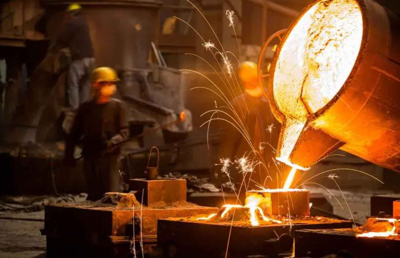
The following visual reference illustrates a representative sand casting production environment. It helps me keep the practical context in view when I design the automation layer, because the final goal is not merely to call a program, but to support real foundry process decisions.
I treat the existing simulation program as the computational core. That program already contains modules for mold filling, solidification, thermal stress, and stress-field mesh processing. My automation layer does not replace those modules. Instead, I wrap them with tools that can read files, classify three-dimensional models, generate a mold, write parameter packages, estimate mesh size, invoke solvers, and read engineering status. In this way, the sand casting simulation program keeps its numerical capability, while the user interacts through natural language or a structured form. The automation layer converts the user’s intent into a structured simulation task and then calls deterministic tools to execute the task.
1. Why sand casting simulation needs an automation layer
Numerical simulation of sand casting can predict mold filling, solidification, temperature fields, stress fields, and defect formation. It can help identify shrinkage cavities, shrinkage porosity, cracks, and other defects before a trial casting is made. In my work, I have seen that simulation can reduce trial runs and shorten process optimization cycles. It can also provide a basis for gating and feeding system design, cooling condition selection, and structural improvement. However, the practical use of simulation is often limited by the preparation burden. Many existing programs are file-driven. They require many inputs, impose strong format constraints, and have complex stage dependencies. Units and orders of magnitude are easy to misplace. Process engineers must repeatedly switch among geometry models, material thermophysical properties, heat transfer boundaries, mesh controls, and multi-stage calculation relationships. If one path, parameter, or stage association is wrong, the calculation may fail or the result may be unusable.
I found that this problem does not necessarily come from insufficient solver capability. It comes more from the complexity of the engineering usage environment. The user may know the process, but still struggle with the input structure. The user may understand heat transfer, but still make a unit error in the interface heat transfer coefficient. The user may know the alloy, but still select the wrong material file. Therefore, I focused on the engineering usage layer. My goal was to build a lightweight encapsulation that preserves the existing sand casting simulation kernel and adds automated invocation, parameter organization, rationality checking, batch scheduling, and result aggregation.
2. OpenClaw, MCP, and skill-based task organization
I position OpenClaw as the interaction and scheduling layer. OpenClaw receives natural language or form-based process information, converts the user’s intent into a structured simulation task, and requests confirmation at critical steps. Unlike a pure chat tool, OpenClaw does not stop at generating explanatory text. It decomposes the task into executable steps and assigns those steps to deterministic tools. MCP is the model context protocol. I use it to create standardized connections between the language model and external files, scripts, databases, or professional software. Through MCP, external programs can be called as tools. A skill is a task-oriented procedural module. It describes the execution steps, invocation rules, and precautions for a certain class of tasks. I further encapsulate common operations in sand casting simulation as a skill. This skill organizes three-dimensional model classification, mold generation, parameter checking, solver invocation, and result aggregation into a fixed workflow. OpenClaw can then call MCP tools in a predefined order. This approach preserves the flexibility of tool calls while reducing the burden on the user to repeatedly enter operation details.
From a layered perspective, my system has three layers. The user interaction layer is handled by OpenClaw. It is responsible for natural language input, task parsing, and interactive confirmation. The tool invocation layer is handled by OpenClaw with loaded MCP tool services. It is responsible for file reading, model classification, parameter writing, and program invocation. The computation execution layer is handled by the existing sand casting simulation program. It is responsible for numerical calculations such as mold filling, solidification, and thermal stress. Table 1 summarizes the roles and responsibilities of each layer.
| Layer | Main component | Responsibilities | Typical outputs |
|---|---|---|---|
| User interaction | OpenClaw | Natural language input, intent parsing, interactive confirmation, risk explanation | Structured task description, confirmation records |
| Tool invocation | OpenClaw with MCP tool services | File reading, 3D model classification, parameter writing, program invocation, status reading | Tool call logs, parameter packages, mesh estimates |
| Computation execution | Existing sand casting simulation program | Mold filling, solidification, thermal stress, defect prediction | Temperature fields, flow fields, stress fields, defect statistics |
3. Automated modeling and task invocation
Automated encapsulation requires converting user-provided process information into a stable data structure. I designed the automated modeling module with clear inputs, processing steps, and outputs. For mold filling calculation, the key parameters include the casting model, pouring direction, pouring temperature, material, filling termination fraction, pouring method, number of threads, and result output interval. For solidification calculation, the user must also provide the solidification termination condition, cooling termination temperature or time, and the association with the previous filling stage. For thermal stress calculation, additional information is needed, such as the stress analysis mesh, the thermal history association stage, and the calculation accuracy. Table 2 lists the main input parameters for each stage.
| Calculation stage | Required parameters | Optional or inferred parameters | Stage dependency |
|---|---|---|---|
| Mold filling | Casting model, pouring direction, pouring temperature, material, filling termination fraction, pouring method, thread count, output interval | Initial mold temperature, air cooling boundary, default heat transfer curve | None |
| Solidification | Solidification termination condition, cooling termination temperature or time, material properties, interface heat transfer | Mold preheat temperature, cooling curve, default yieldability parameters | Reads filling stage result |
| Thermal stress | Stress analysis mesh, thermal history association stage, calculation accuracy | Tetrahedral mesh size, stress output interval | Reads solidification stage result |
In a traditional manual workflow, the user must decide which three-dimensional model corresponds to the casting, runner, riser, chill, or mold. I implemented an MCP tool that uses model name hints and geometric bounding box information to identify the role of each model. When the classification confidence is insufficient, the system keeps a manual confirmation entry. For tasks where no mold model is provided, the system can generate an aligned mold model from the outer bounding box of the casting or gating system. This satisfies the needs of subsequent mesh generation and heat transfer boundary setting. The mold generation rule can be expressed as follows. For a bounding box with lengths \(L_x\), \(L_y\), and \(L_z\), and a user-confirmed offset \(\delta\), the mold bounding box is:
$$L_{mold,x} = L_{casting,x} + 2\delta$$
$$L_{mold,y} = L_{casting,y} + 2\delta$$
$$L_{mold,z} = L_{casting,z} + 2\delta$$
The gate side is determined by the pouring direction. In my current implementation, I use the rule that the gate side corresponds to the mold outer surface whose normal is opposite to the pouring gravity direction. For example, when the liquid metal enters vertically downward, the gate side corresponds to the upper surface of the mold. This side is not expanded by default, or it uses a separate offset. The other directions are generated according to the user-confirmed offset. This rule is easy to explain, and it is also easy to communicate to the user during interaction.
When generating calculation content automatically, I use stable templates and structured parameters to reduce manual editing. The MCP parameter writing tool can organize the confirmed sub-steps into a complete CAE parameter package. This package includes engineering control parameters, geometry part lists, interface heat transfer relationships, air heat transfer boundaries, mesh data, process configuration, default heat transfer curves, default yieldability parameters, and automated task records. The automated task record stores the structured parameters, material data, program location, and mesh estimation result used in the current task. It can be used for later tracking and for reproducing experiments.
Multi-stage calculation is organized through sibling subtasks. The filling, solidification, and thermal stress stages each retain their own control parameters. When solidification needs to read the filling result, the solidification stage record points to the previous filling subtask. When thermal stress needs to read the solidification temperature history, the thermal stress stage record points to the solidification subtask and specifies the corresponding stress analysis mesh. This makes the originally scattered stage dependencies explicit and reduces the probability of errors caused by manually copying paths and rewriting names.
After the calculation content is generated, the system calls the corresponding CAE calculation program according to the stage type. It reads the engineering status before and after running. Before solving, it mainly checks whether the control parameters, three-dimensional geometry models, material data, and program location are complete. After solving, it mainly checks whether the key output files of each stage are generated correctly. These files include mesh records, casting mesh, filling fields, solidification temperature fields, and defect criteria. If a stage fails, the system returns the failed stage, the running command, the exit code, the tail of the log, possible causes, and retry suggestions.
4. Parameter-assisted configuration and rationality checking
The goal of the parameter-assisted checking module is to convert process experience, file constraints, and solver operating constraints into executable rules. The rules themselves do not all need to rely on complex machine learning models. Many high-value checks can be completed through range judgment, order-of-magnitude judgment, path existence judgment, and stage dependency judgment. The value of OpenClaw is that it turns the check results into prompts that engineers can easily understand and organizes necessary secondary confirmation for high-impact parameters. I divided the inspection rules into six categories: initial temperature rules, material thermophysical property rules, heat transfer boundary rules, geometry and mold rules, finite difference mesh size rules, and tetrahedral mesh size rules. Table 3 gives examples of these rules.
| Inspection object | Inspection rule | Prompt content |
|---|---|---|
| Initial temperature | Read the material library. The preset pouring temperature must be higher than the liquidus of the material and have a reasonable superheat. The mold preheat temperature must be within a reasonable range. | The pouring temperature is low, which may cause incomplete filling or premature solidification. Check the material liquidus and pouring temperature. The mold preheat temperature is too high. Check engineering rationality. |
| Material file | The casting and mold material files must exist. The material thermophysical properties must satisfy common orders of magnitude. | The specified material file was not found. Select from the material library or supplement and modify the material data. |
| Interface and environment heat transfer coefficient | The heat transfer coefficient must conform to engineering experience. | The interface heat transfer parameter may be unreasonable. Confirm the unit and magnitude. |
| Mold offset | Except for the gate side, the mold must cover the casting. | The mold offset is too small, which may cause abnormal finite difference mesh or boundary conditions. |
| Finite difference mesh count | The default upper limit is \(1\,000\,000\) cells. | The estimated mesh count exceeds the default upper limit. Increase the mesh size, or confirm that a larger mesh count is allowed despite longer calculation time. |
| Tetrahedral mesh count | The default upper limit is \(200\,000\) tetrahedra. | The estimated tetrahedral count is large, which may affect thermal stress calculation time. |
Mesh size directly affects calculation stability, running time, and memory consumption. Therefore, I estimate it before solving. For a finite difference mesh, the number of cells can be estimated from the mold outer bounding box size and the minimum mesh thickness. When the user does not specify the mesh thickness, the system back-calculates a suggested value from the default mesh upper limit so that the estimated mesh count does not exceed the limit. In my current project, the default finite difference mesh upper limit is \(1\,000\,000\) cells. After actual mesh generation, the system reads the mesh status again to confirm whether the actual mesh count is reasonable. The finite difference mesh size can be estimated by:
$$N_x = \left\lceil \frac{L_x}{h} \right\rceil, \quad N_y = \left\lceil \frac{L_y}{h} \right\rceil, \quad N_z = \left\lceil \frac{L_z}{h} \right\rceil$$
$$N = N_x N_y N_z$$
where \(L_x\), \(L_y\), and \(L_z\) are the dimensions of the mold bounding box in three directions, \(h\) is the mesh size, and \(N\) is the estimated mesh count. This estimate is used to judge whether the mesh size exceeds the default protection limit before the real calculation. For a thermal stress tetrahedral mesh, the system can estimate the number of tetrahedra from the STL surface mesh boundary range and the target partition number. The default protection limit is \(200\,000\) tetrahedra. A simple estimate is:
$$N_{tet} \approx \frac{V_{part}}{V_{tet}}$$
where \(V_{part}\) is the volume of the part to be meshed and \(V_{tet}\) is the average volume of a single tetrahedron. In practice, I also use the surface area and the target edge length to refine the estimate. The purpose is not to replace a real mesher but to warn the user before a very large thermal stress calculation is launched.
Some parameters in sand casting simulation have a significant impact on the calculation result and resource consumption. The automation system should confirm these parameters before writing files or executing external programs. These parameters include the solution workflow, STL classification result, pouring direction, gate side, mold offset, material name, pouring temperature, finite difference mesh settings, tetrahedral mesh settings, solver path, output path, overwrite strategy, and whether to actually execute the external program. The purpose of the confirmation mechanism is not to increase user burden. It is to make the risk points that were previously hidden in complex files explicit.
In the interaction strategy, OpenClaw adopts a default suggestion, risk explanation, and one-time confirmation process. For example, when the estimated finite difference mesh count approaches the upper limit, the system prompts the suggested minimum mesh size parameter, explains that this value is used to control the mesh count, and asks whether the user accepts it. When the three-dimensional model name cannot clearly determine the role, the system displays the classification basis and confidence and requires the user to confirm the casting, runner, or mold role. I found that this approach reduces silent errors and keeps the engineer in control of high-impact decisions.
5. Numerical models behind the sand casting simulation
Although my main contribution is the automation and parameter assistance layer, I still rely on the underlying numerical models of the existing sand casting simulation program. For mold filling, the liquid metal flow is governed by the conservation of mass and momentum. The continuity equation is:
$$\frac{\partial \rho}{\partial t} + \nabla \cdot (\rho \mathbf{u}) = 0$$
The momentum equation for an incompressible or weakly compressible flow can be written as:
$$\rho \left( \frac{\partial \mathbf{u}}{\partial t} + \mathbf{u} \cdot \nabla \mathbf{u} \right) = -\nabla p + \mu \nabla^2 \mathbf{u} + \rho \mathbf{g}$$
where \(\rho\) is density, \(\mathbf{u}\) is velocity, \(t\) is time, \(p\) is pressure, \(\mu\) is dynamic viscosity, and \(\mathbf{g}\) is gravitational acceleration. During filling, the volume-of-fluid or a similar free-surface tracking method is used to capture the melt front. The filling termination fraction is defined as the ratio of filled volume to cavity volume:
$$f_{fill} = \frac{V_{filled}}{V_{cavity}}$$
For solidification, the heat conduction equation with phase change is solved:
$$\rho c_p \frac{\partial T}{\partial t} = \nabla \cdot (k \nabla T) + Q$$
where \(T\) is temperature, \(c_p\) is specific heat capacity, \(k\) is thermal conductivity, and \(Q\) is the latent heat source term. The latent heat is often handled by an effective specific heat or an enthalpy method. The solid fraction \(f_s\) is commonly expressed as:
$$f_s = \frac{T_L – T}{T_L – T_S}, \quad T_S \le T \le T_L$$
where \(T_L\) is the liquidus temperature and \(T_S\) is the solidus temperature. For thermal stress, the stress-strain relationship can be written as:
$$\boldsymbol{\sigma} = \mathbf{C} : \left( \boldsymbol{\varepsilon} – \boldsymbol{\varepsilon}^{th} \right)$$
where \(\boldsymbol{\sigma}\) is the stress tensor, \(\mathbf{C}\) is the elastic stiffness tensor, \(\boldsymbol{\varepsilon}\) is the total strain tensor, and \(\boldsymbol{\varepsilon}^{th}\) is the thermal strain tensor. The equivalent stress is often used for post-processing:
$$\sigma_{eq} = \sqrt{\frac{1}{2} \left[ (\sigma_1 – \sigma_2)^2 + (\sigma_2 – \sigma_3)^2 + (\sigma_3 – \sigma_1)^2 \right]}$$
For shrinkage cavity and shrinkage porosity prediction, I use the defect criteria provided by the existing solver. A common criterion is based on the thermal gradient \(G\) and the cooling rate \(R\):
$$G = \left| \nabla T \right|, \quad R = \left| \frac{\partial T}{\partial t} \right|$$
The feeding resistance or defect index can be expressed as a function of \(G\) and \(R\), such as \(G/\sqrt{R}\) or \(G \cdot \sqrt{R}\), depending on the alloy and the specific criterion. The system does not alter these criteria. It only organizes the parameters and extracts the resulting defect volumes.
6. Implementation and validation of the automated workflow
I validated the automated workflow with a stepped test block. The system starts from three-dimensional models and process parameters and sequentially completes model classification, mold generation, parameter package writing, mesh estimation, filling calculation, solidification calculation, thermal stress calculation, and result aggregation. The input parameters include casting material, mold material, pouring temperature, pouring direction, mold offset, filling termination fraction, solidification termination condition, output interval, thread count, and program path. In this validation case, the material was ZG35CrMo cast steel, the pouring temperature was \(1\,570^\circ\mathrm{C}\), the mold was resin sand, and the mesh size was \(10.53\,\mathrm{mm}\).
With DeepSeek-V4-Flash as the driving model, the system completed the continuous invocation from process requirement input to post-processing result aggregation. The interaction record omitted local paths, command lines, and redundant logs. The important point is that the automation layer connected model processing, parameter configuration, stage invocation, and result aggregation into one task chain. Its value was not to change the calculation result itself but to reduce the manual work of finding files, filling parameters, and confirming stage dependencies.
To illustrate the configuration efficiency change and the adaptability of the system to different base models, I compared several base models with the traditional manual method. The time here mainly refers to the typical task configuration and process organization time, not the underlying computation time. Under the same geometry model, same material, and same process conditions, different base models could drive the three-stage simulation workflow, but the operation efficiency and parameter configuration quality differed. Table 4 summarizes the operation records.
| Metric | Traditional manual method | DeepSeek-V4-Flash | Kimi K2.7 code | GLM 5.2 | Qwen 3.8 |
|---|---|---|---|---|---|
| Working time | 20 min | 4.5 min | 3.3 min | 4.3 min | 10.4 min |
| Parameter check prompts | Not applicable | 1 | 1 | 1 | 1 |
| Manual interventions to correct errors | Not applicable | 0 | 0 | 0 | 0 |
From the perspective of engineering parameter settings and simulation execution results, DeepSeek-V4-Flash, GLM-5.2, and Qwen-3.8 all used a casting-to-sand mold heat transfer coefficient curve that varied with temperature. Compared with a constant heat transfer coefficient, this can describe the interfacial heat transfer behavior in different temperature stages in more detail. Kimi-K2.7code used a constant heat transfer coefficient of \(500\,\mathrm{W/(m^2\cdot K)}\) and configured a finer mesh. Although the parameters were simplified, it still completed the filling, solidification, and thermal stress calculations. GLM-5.2 used solid fraction control for the solidification termination condition and also obtained complete results. Qwen-3.8 completed all calculations and generated a complete simulation analysis report, making the task delivery the most comprehensive. Overall, the base models differed in the choice of heat transfer boundary, mesh accuracy, and calculation control parameters, but all could automatically complete the full simulation workflow.
For the stepped test block, I organized the post-processing results in a unified way. The geometry and mesh results showed that the casting had a clear stepped thickness variation. The finite difference mesh represented the casting body, runner, and riser contours. The tetrahedral mesh used for thermal stress analysis had relatively fine local refinement at the gating system, the sprue root, and geometric transition regions. This helped describe temperature gradients and stress changes at structural discontinuities. During filling, the metal first flowed along the sprue and runner and entered the stepped test block cavity through three ingates. In the early filling stage, high-velocity regions were mainly concentrated near the sprue, runner, and ingates. As filling progressed, the metal gradually spread over the stepped test block surface and expanded into thick regions. In the later filling stage, the casting body was basically filled, and the velocity field became relatively uniform, with higher velocities remaining only in the gating system and local connection regions.
During solidification, the overall temperature of the casting gradually decreased. In the early solidification stage, high-temperature regions were mainly concentrated near the thick steps, runners, and risers. Thin-walled regions and edges cooled faster, showing obvious cooling differences between thick and thin regions. The equivalent stress was unevenly distributed in the casting body and gating and feeding system. Higher stress regions mainly appeared at the end and root of the shaped riser, the ingate connection positions, and geometric mutation regions. This was mainly related to temperature gradients during cooling, shrinkage differences in different regions, and structural constraints. The thick-thin transition and runner connection regions were prone to local stress concentration because of geometric continuity changes. The shaped riser and its root region also showed higher stress levels because of different cooling paths and constraint conditions. These results can provide reference for subsequent process analysis, such as fillet transition optimization, local cooling condition adjustment, gating and feeding system removal sequence design, and hot cracking risk assessment.
For shrinkage cavity and shrinkage porosity prediction, the risk was mainly concentrated on the upper surface of the casting, thick regions, and local hot spots near the gating and feeding system. This was basically consistent with the characteristics of slow cooling and long high-temperature duration in thick regions shown by the solidification temperature field. The post-processing statistics showed that the total shrinkage cavity volume was \(938.18\,\mathrm{cm^3}\) and the total shrinkage porosity volume was \(3136.39\,\mathrm{cm^3}\). Table 5 summarizes the defect statistics for the stepped test block. The system not only automatically organized the shrinkage cavity and shrinkage porosity distribution but also extracted defect count, defect volume, and internal defect statistics. This provides a quantitative basis for subsequent process evaluation.
| Defect type | Total volume (cm³) | Main location | Related process feature |
|---|---|---|---|
| Shrinkage cavity | 938.18 | Upper surface, thick regions, local hot spots | Slow cooling in thick sections, riser feeding limitation |
| Shrinkage porosity | 3136.39 | Thick steps, gating and feeding system vicinity | Dispersed solidification shrinkage, insufficient feeding |
| Total defect volume | 4074.57 | Combined hot spot regions | Thermal gradient and cooling rate distribution |
7. Error parameter identification
I validated the parameter-assisted checking module with a second set of cases. Using DeepSeek-V4-Flash as the base model, I kept the geometry model unchanged and constructed anomalies such as pouring temperature below the material liquidus, unreasonable heat transfer coefficient, too small mold offset, over-dense mesh, and missing material data. The system should intercept these problems before writing calculation content, generating the mesh, or invoking the program, and give modification suggestions that engineers can directly understand. Table 6 lists the anomaly cases and the system prompts.
| Anomaly case | Inspection rule triggered | System prompt |
|---|---|---|
| Pouring temperature below liquidus | Initial temperature rule | The pouring temperature is lower than the material liquidus. Check the material liquidus and pouring temperature. Increase superheat or select the correct material. |
| Unreasonable heat transfer coefficient | Interface and environment heat transfer rule | The interface heat transfer coefficient magnitude is abnormal. Confirm the unit and the intended interface condition. |
| Too small mold offset | Geometry and mold rule | The mold offset is too small. The mold may not fully cover the casting, which may cause abnormal finite difference mesh or boundary conditions. |
| Over-dense mesh | Finite difference mesh size rule | The estimated mesh count exceeds the default upper limit. Increase the mesh size or confirm that a larger mesh count is allowed. |
| Missing material data | Material thermophysical property rule | The specified material file was not found. Select from the material library or supplement the material data. |
The parameter checking module converted low-temperature pouring, abnormal heat transfer coefficient magnitude, too small mold size, excessive mesh size, and missing material data into clear prompts. It could also identify multiple parameter anomalies at the same time. Compared with manual item-by-item checking, these prompts are closer to the location where the error occurs. They expose risks before solving and reduce invalid calculations. In my view, this is one of the most practical benefits of the automation layer for sand casting simulation. It does not require the solver to be changed, but it prevents many common input mistakes from reaching the solver.
8. Automated orthogonal experiment validation
To validate the continuous invocation ability of the automated workflow for multiple process parameter sets of a complex structural casting, I constructed a \(2 \times 3\) orthogonal experiment for a bearing housing casting. The experiment considered superheat \(T\) and casting material as factors. The superheat levels were \(20^\circ\mathrm{C}\), \(50^\circ\mathrm{C}\), and \(80^\circ\mathrm{C}\). The materials were HT250 and 16Mn steel. The remaining geometry, material, mold offset, calculation control, and result extraction criteria were kept consistent. The system automatically organized calculation tasks according to the parameter combinations and extracted shrinkage cavity and shrinkage porosity distributions and casting porosity volume statistics after calculation. Table 7 lists the factors and levels of the orthogonal experiment.
| Factor | Level 1 | Level 2 | Level 3 |
|---|---|---|---|
| Material | 16Mn steel | HT250 | — |
| Superheat \(T\) | \(20^\circ\mathrm{C}\) | \(50^\circ\mathrm{C}\) | \(80^\circ\mathrm{C}\) |
The results showed that the material type determined the base level of shrinkage cavity and shrinkage porosity, while superheat determined the development degree of defects in that material. As superheat increased from \(20^\circ\mathrm{C}\) to \(80^\circ\mathrm{C}\), the shrinkage cavity volume of both materials increased, while the shrinkage porosity volume decreased. The defect composition showed a trend of changing from dispersed shrinkage porosity to concentrated shrinkage cavity. Based on the sum of shrinkage cavity and shrinkage porosity volumes, the total defect volume of 16Mn steel increased from \(17\,011.56\,\mathrm{cm^3}\) to \(18\,493.97\,\mathrm{cm^3}\). The total defect volume of HT250 decreased from \(11\,089.94\,\mathrm{cm^3}\) to \(8\,288.80\,\mathrm{cm^3}\) and tended to stabilize in the range of \(50^\circ\mathrm{C}\) to \(80^\circ\mathrm{C}\). Table 8 gives the defect volume comparison.
| Material | Superheat (°C) | Shrinkage cavity volume (cm³) | Shrinkage porosity volume (cm³) | Total defect volume (cm³) |
|---|---|---|---|---|
| 16Mn steel | 20 | — | — | 17 011.56 |
| 16Mn steel | 50 | — | — | — |
| 16Mn steel | 80 | — | — | 18 493.97 |
| HT250 | 20 | — | — | 11 089.94 |
| HT250 | 50 | — | — | — |
| HT250 | 80 | — | — | 8 288.80 |
The focus of this experiment was not to give a unique optimal process but to test whether the automated encapsulation layer could stably complete batch task generation, parameter writing, program invocation, and result aggregation. Compared with manually copying projects, modifying parameters, and collecting statistics group by group, the automated workflow ensured that all six cases used the same input criteria and the same post-processing rules. This reduced human input differences and made it easier to connect defect volume, calculation status, and abnormal prompts to the process parameter screening process. In my view, this is a key step toward using sand casting simulation in a more data-driven way.
9. Discussion
Compared with secondary development aimed at the underlying numerical format, my method is more suitable for scenarios where an existing calculation program already has stable capability but a high usage threshold. Its advantage is that it does not destroy the original program structure. It can reuse the existing material library, example projects, and calculation modules. At the same time, it improves parameter configuration efficiency and process traceability through the automation layer. I found that this is a practical compromise between a full software rewrite and a pure manual workflow.
The method still has limitations. The parameter inspection rules depend on the material database, template experience, and historical case accumulation. When the rule coverage is insufficient, complex errors may still be missed. Natural language input may also be ambiguous, so high-impact parameters still require manual confirmation. Automatic mold generation and fallback mesh are suitable for process verification, but production-level simulation still needs to be reviewed according to actual process and mesh quality requirements. Automatic result aggregation still depends on the model’s ability to understand images and logs, which needs further strengthening.
Future work can proceed in three directions. First, I can expand the material and process template library to cover more process types such as sand casting, permanent mold casting, low-pressure casting, and investment casting. Second, I can associate parameter inspection rules with historical successful cases to form a more stable recommendation mechanism. Third, I can improve the automatic result aggregation module so that temperature fields, liquid fraction, solidification time, and thermal stress results can automatically generate standardized reports.
10. Conclusion
I constructed a method that uses an existing sand casting simulation program as the computational core, OpenClaw as the interaction and scheduling entry, and a skill plus MCP tool service to connect three-dimensional model recognition, mold generation, parameter package writing, mesh estimation, program invocation, and engineering status reading. Around the input system of this type of program, I organized the relationships among engineering control parameters, heat transfer relationships, mesh settings, material data, and stage outputs. I established parameter inspection rules for materials, temperature, inflow velocity, mold initial temperature, heat transfer boundaries, mesh size, stage relationships, and program locations. These rules can find common configuration problems before calculation content is written and before the program is run. They also reduce the risk of misconfiguration through interactive confirmation.
The stepped test block case validated the effectiveness of the system in configuration efficiency, abnormal parameter identification, and batch invocation. The typical task configuration time was reduced from \(20\,\mathrm{min}\) to \(4.5\,\mathrm{min}\). The abnormal parameter case showed that the workflow can give prompts for pouring temperature, heat transfer coefficient, mold size, mesh size, and material data problems. The orthogonal experiment case showed that the automation layer can stably complete batch invocation and defect volume statistics under multiple parameter combinations. Therefore, this method can serve as a lightweight encapsulation solution for existing sand casting simulation programs when they are used by process engineers. It preserves the trusted numerical kernel while making the sand casting simulation workflow more accessible, more consistent, and more traceable.