
In the intricate world of manufacturing high-integrity metal components, the lost wax casting process stands out for its ability to produce complex, near-net-shape parts with excellent surface finish. However, the very complexity that defines this process also governs its thermal history, which ultimately dictates the final microstructure, mechanical properties, and soundness of the cast component. As a practitioner deeply involved in process development and simulation, I have found that one of the most critical, yet challenging, pieces of data to obtain is the accurate cooling curve during the solidification phase of a lost wax casting. This curve is not merely a temperature-time plot; it is the fundamental signature of the casting process, encoding the effects of alloy properties, mold material, interfacial conditions, and boundary heat transfer. Its accurate acquisition is paramount for the inverse calculation and optimization of simulation parameters in software like ProCAST, which we rely on to predict defects, optimize risers, and reduce costly prototyping cycles.
The journey to a reliable simulation often begins and ends with thermal data. While commercial simulation packages provide powerful solvers for fluid flow, heat transfer, and stress analysis, their predictive accuracy is heavily contingent upon the input parameters that define the physical reality of the process. For a lost wax casting simulation, this reality is described by a set of over 30 parameters. A significant subset, including interfacial heat transfer coefficients (IHTC) and boundary conditions like convection and radiation coefficients, cannot be simply looked up in a handbook. They are dynamic, process-dependent variables. The ProCAST inverse solver module offers a pathway to determine these elusive parameters, but it requires one crucial input: the experimental cooling curve of the casting itself. Without this empirical anchor, simulation remains an educated guess. This article details, from a first-hand perspective, the methodologies, challenges, and solutions for measuring high-precision cooling curves within steel investment castings, a task essential for bridging the gap between digital simulation and foundry reality.
The Foundational Role of Cooling Curves in Lost Wax Casting Simulation
To appreciate the measurement challenge, one must first understand what the cooling curve represents. During solidification of a metal, heat is extracted through the mold. The rate of this extraction, plotted as temperature against time, reveals plateaus (for pure metals) or changes in slope (for alloys) corresponding to latent heat release at the liquidus and solidus temperatures. The shape of this curve between these points is governed by the Fourier heat conduction equation:
$$
\rho c_p \frac{\partial T}{\partial t} = \nabla \cdot (k \nabla T) + \dot{q}
$$
Where \( \rho \) is density, \( c_p \) is specific heat, \( k \) is thermal conductivity, \( T \) is temperature, \( t \) is time, and \( \dot{q} \) is the internal heat source term (latent heat). In the context of lost wax casting, the boundary conditions for this equation are exceptionally complex. The ceramic shell, born from repeated slurry and stucco coatings, has anisotropic thermal properties. The interface between the hot metal and the pre-heated shell involves a contact resistance quantified by the IHTC, \( h_{int} \), defined as:
$$
q = h_{int} (T_{casting} – T_{mold})
$$
where \( q \) is the heat flux. This coefficient is influenced by surface roughness, air gap formation upon solidification shrinkage, and even the composition of the shell face coat. Externally, the shell radiates heat to its surroundings and convects heat to the ambient air within the pouring cluster. Accurately defining these \( h_{int} \), convection (\( h_{conv} \)), and radiation (\( \epsilon \)) parameters is the key to a faithful simulation. The inverse method uses the experimental cooling curve \( T_{exp}(t) \) to iteratively adjust these unknown parameters in the simulation until the simulated cooling curve \( T_{sim}(t) \) matches the measured one, minimizing an objective function \( F \):
$$
F(h_{int}, h_{conv}, \epsilon) = \sum_{i=1}^{n} [T_{sim}(t_i) – T_{exp}(t_i)]^2
$$
Therefore, the precision of the measured \( T_{exp}(t) \) directly dictates the reliability of the inversely calculated parameters, and consequently, the predictive power of the simulation for all future castings using that shell system and alloy.
| Parameter Category | Specific Parameters | Typical Source / Determination Method | Challenge in Lost Wax Casting |
|---|---|---|---|
| Material Properties | Density (ρ), Specific Heat (cp), Thermal Conductivity (k) of alloy and shell. | Material databases, Handbook values, DSC/TGA testing. | Shell properties are composite and process-dependent. |
| Initial Conditions | Pouring Temperature, Shell Preheat Temperature. | Direct pyrometer or thermocouple measurement. | Shell temperature can vary within a cluster. |
| Critical Unknowns (for Inverse Calculation) | Interface Heat Transfer Coefficient (IHTC). | Inverse calculation using cooling curves. | Varies with time, location, and shell/metal conditions. |
| Critical Unknowns (for Inverse Calculation) | Boundary Conditions: Convection Coefficient, Radiation Emissivity. | Inverse calculation or empirical estimation. | Highly dependent on cluster configuration and furnace environment. |
Designing the Measurement Experiment for Lost Wax Casting
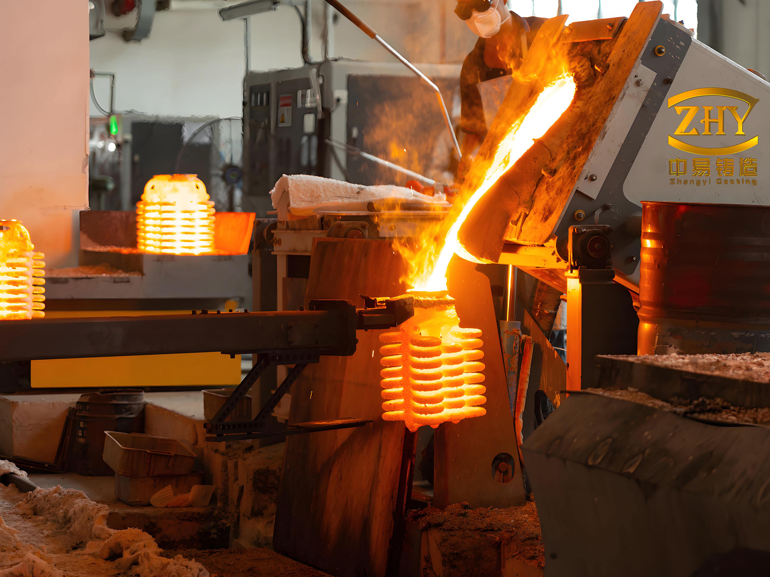
The goal is to capture the temperature at a critical point inside a solidifying steel casting from above the pouring temperature down to well below its solidus. For a typical low-carbon steel like ZG310-570 with a melting range of approximately 1416-1491°C, this means measuring from ~1550°C down to ~1200°C over a period that can last 30 minutes or more. The first step is to design a representative test geometry. To systematically understand cooling behavior across different section thicknesses and orientations, a stepped plate or block model is ideal. This allows for the placement of thermocouples at strategic “upper, middle, and lower” locations corresponding to varying thermal moduli. Isolating these measurement points onto separate, identical patterns within a cluster is often necessary to avoid interference between multiple thermocouple assemblies and to ensure each sensor is encapsulated correctly.
The core of the measurement system is the thermocouple. The principle is based on the Seebeck effect: a voltage is generated at the junction of two dissimilar conductors when a temperature gradient exists. For lost wax casting of steels, the environment is punishing—oxidizing, high-temperature, and physically abrasive. Therefore, the choice of thermocouple type is critical. Type B (Pt-30%Rh/Pt-6%Rh) and Type K (Ni-Cr/Ni-Al) thermocouples are the primary candidates due to their high upper-temperature limits and oxidation resistance in air. Their relevant characteristics are summarized below:
| Thermocouple Type | Composition | Typical Range (Continuous) | Advantages for Lost Wax Casting | Disadvantages for Lost Wax Casting |
|---|---|---|---|---|
| B-Type | Pt-30%Rh / Pt-6%Rh | 870°C to 1700°C | Highest temperature capability; stable in oxidizing atmospheres; minimal drift. | Lower sensitivity (~10 µV/°C); high cost. |
| K-Type | Ni-Cr / Ni-Al | -200°C to 1260°C (up to 1370°C short-term) | High sensitivity (~41 µV/°C); lower cost; wide temperature range. | Can drift in oxidizing atmospheres above ~1000°C; susceptible to “green rot”. |
For measuring steel castings with pouring temperatures up to 1650°C, Type B is often the safer choice for long-term stability, though Type K can be used with the understanding that it may be a consumable item. The thermocouple wires must be connected to compensating extension wires of the correct type, which in turn feed into a high-speed, multi-channel data acquisition system capable of scanning at a rate appropriate to capture the dynamics of solidification (e.g., 1-10 Hz).
The Crucial Challenge: Thermocouple Encapsulation and Survival
This is where the unique aspects of lost wax casting create significant hurdles. Unlike sand casting where a thermocouple can be pushed into the mold sand, the ceramic shell in lost wax casting is rigid, thin, and produced through a multi-step build-up process. Furthermore, the shell is subjected to a high-temperature burnout (typically 950-1050°C for 2-4 hours) before pouring, and the cluster radiates intense heat during pouring, creating a hostile ambient environment for unprotected wires.
A bare thermocouple will not survive. It requires a robust protection system with the following attributes: excellent thermal conductivity for fast response, high refractoriness to withstand molten steel, sufficient mechanical strength to handle handling and metal static pressure, and chemical inertness. High-purity alumina (Al2O3, >99%) tubes and sleeves are the material of choice. The encapsulation strategy is a delicate balance between measurement fidelity and sensor survival. The ideal scenario is for the thermocouple’s hot junction to be in direct, intimate contact with the solidifying metal. This can be attempted by using a multi-layer protection system: an outer alumina protection sheath is fixed within the shell, an inner alumina insulator tube holds the two thermocouple wires, and at the very tip, the welded bead of the thermocouple wires is exposed, sealed in place only by a small plug of fine-grain refractory cement. This cement must be porous enough to allow metal infiltration to contact the bead upon pouring.
The thermal response of such an assembly can be modeled considering the series of thermal resistances. The overall time constant \( \tau \) affecting the measurement is a function of the thermal properties and geometry of each layer. For a simplified model, the dominant resistance is often the cement plug. The goal is to minimize its thickness \( L_{cem} \) and maximize its effective conductivity \( k_{eff} \). The heat flux \( q \) to the bead is approximated by:
$$
q \approx \frac{k_{eff}}{L_{cem}} (T_{metal} – T_{bead})
$$
This method yields high-fidelity data, as the bead is in near-direct contact with the metal. However, in practice, the thermocouple bead is extremely vulnerable. The intense thermal shock from the molten steel, combined with potential chemical reaction or erosion, often leads to failure within 20-30 minutes of measurement—sometimes just after the critical solidification period. Alternative, more protective sealing methods using thicker ceramic plugs increase survivability but introduce a larger thermal lag, effectively low-pass filtering the true cooling curve and obscuring critical inflection points. Finding the optimal refractory cement composition and application technique is a key practical art in lost wax casting thermometry.
Strategic Placement Within the Lost Wax Casting Process Flow
The second major hurdle is the physical placement and fixing of the thermocouple assembly within the fragile ceramic shell. The process flow for integrating a thermocouple differs depending on whether the target is the shell temperature or the casting temperature.
For Shell Temperature Measurement: The strategy is to create a dedicated cavity within the shell wall. After a sufficient thickness of shell (e.g., >5 mm) has been built up on the wax pattern, the assembly process is paused. A thin alumina tube (the future thermocouple guide) is inserted into a pre-designed location on the pattern assembly. The subsequent slurry and stucco coats are then carefully applied, embedding and locking this tube in place. After dewaxing and firing, this tube creates an open channel from the outside of the fired shell to a point embedded within its wall thickness. During the experiment, a pre-assembled and encapsulated thermocouple is simply inserted into this guide tube until it seats at the bottom, ready to measure the shell’s internal temperature during pour and cooling.
For Casting Temperature Measurement: Here, the thermocouple tip must reside within the actual mold cavity. The procedure is more involved. A robust outer alumina protection sheath is inserted directly into the wax pattern at the desired measurement point during wax assembly. The entire wax tree, with sheaths protruding, then goes through the standard shell building process. The shell material completely envelops and grips the sheath. After dewaxing, the sheath remains firmly anchored in the shell, with its open tip now forming part of the mold cavity. The shell is then fired. Crucially, the sensitive thermocouple itself is not subjected to the firing cycle. Only the empty, robust sheath is. Just before pouring, the pre-calibrated thermocouple assembly is inserted from the back of the cluster into this pre-positioned sheath, where it is secured. This method elegantly solves the dual problems of accurate placement and avoiding pre-degradation of the thermocouple during the high-temperature shell burnout.
| Measurement Target | Integration Point in Process | Key Advantage | Key Challenge |
|---|---|---|---|
| Shell Temperature | After partial shell build-up. Thermocouple inserted post-firing. | Simple; thermocouple not exposed to burnout; easy replacement. | Measures shell interior, not the exact metal/shell interface. |
| Casting Temperature | During wax assembly. Sheath is built into shell; thermocouple inserted pre-pour. | Direct measurement of metal temperature; sheath protects during shell building and firing. | Complex wax assembly; risk of sheath leaking or breaking during dewaxing; critical insertion step before pour. |
Results, Interpretation, and Application in Simulation
A successful measurement campaign will yield families of curves. Plotting temperature against time for multiple points provides a rich dataset. The shell cooling curves typically show a rapid initial rise upon metal impingement, followed by a slower decline. The casting curves are the crown jewels. For a steel lost wax casting, a high-quality curve will show a clear arrest or change in slope at the liquidus temperature as nucleation begins and dendrites start to form, releasing latent heat. The slope then continues to decrease until the solidus temperature is reached, where another thermal event may be visible, especially if there is a significant freezing range.
Validation of the data’s credibility is essential. A simple but effective check is to compare the maximum recorded temperature at a point in the casting with an independent measurement of the pouring temperature, such as from a quick-immersion thermocouple in the ladle. In a well-designed experiment, these values should be rationally related, accounting for heat loss during transfer and filling. For instance, a ladle temperature of 1600°C might result in a measured peak in the casting of 1540-1560°C, which is physically consistent.
These validated curves are then formatted and fed into the ProCAST inverse calculation module. The process involves defining the known parameters (alloy properties, shell properties from maybe a separate test, pouring temperature) and selecting the unknown parameters (e.g., metal-shell IHTC, shell-air convection coefficient) to be solved for. The software runs an iterative optimization loop, adjusting these unknowns to minimize the difference between the simulated and experimental curves at the corresponding nodal points. The output is a set of optimized parameters that are specific to that alloy-shell system and cluster configuration.
The power of this methodology is that once these parameters are determined from a well-instrumented test casting, they can be applied with much greater confidence to simulate the solidification of new, more complex geometries within the same foundry environment. This directly addresses the “simulation bias” often encountered when using generic parameters. The ability to predict hot spots, shrinkage porosity, and even microstructural features like secondary dendrite arm spacing (SDAS) is significantly enhanced. SDAS, a key indicator of mechanical properties, is related to the local solidification time \( t_f \), which is directly read from the cooling curve between liquidus and solidus:
$$
SDAS = a \cdot (t_f)^n
$$
where \( a \) and \( n \) are alloy-specific constants. An accurate cooling curve provides \( t_f \), enabling prediction of local microstructure and properties.
Conclusion and Forward Look
The accurate measurement of cooling curves in lost wax casting is a sophisticated but indispensable metrology practice for the modern foundry leveraging simulation-driven design. It transforms simulation from a qualitative visualization tool into a quantitative predictive engine. The challenges are significant—surviving the thermal and chemical assault of molten steel, integrating sensors into a delicate ceramic mold, and extracting high-fidelity data from a harsh environment. However, through careful selection of thermocouple types, innovative multi-layer encapsulation strategies using alumina ceramics, and clever placement techniques that leverage the wax pattern and shell-building process itself, these challenges can be overcome.
The methodology described, involving post-firing insertion for shell measurement and pre-placed sheaths for metal measurement, provides a robust framework. The resulting high-precision cooling curves serve as the critical empirical input for inverse parameter estimation, leading to optimized values for interfacial and boundary heat transfer coefficients. This闭环 of measurement and simulation forms the backbone of a reliable digital twin for the lost wax casting process. Future advancements may lie in the use of wireless telemetry systems to simplify data acquisition from within clusters, or in the development of more robust, disposable sensor tips that sacrifice themselves after delivering perfect data. Nevertheless, the fundamental principle remains: to simulate with confidence, one must first measure with precision. In the quest for zero-defect castings and shortened development cycles, mastering the thermal signature of solidification is not just helpful; it is essential.