
I investigate the investment casting route for an AlSiCuSc alloy turbine volute because the component operates under severe thermal cycling and pressure loading. My central objective is not merely to produce a sound shape, but to control filling, solidification, feeding, and porosity formation in a thin-walled spiral geometry with localized heavy sections. I treat numerical simulation as a decision tool rather than a cosmetic verification step. In parallel, I keep the broader family of lost foam castings in view, because lost foam castings offer an alternative approach for complex metal shapes, and the process physics of lost foam castings often provide useful contrasts with investment casting. However, my experimental work is focused on investment casting, and I use simulation to reduce trial-and-error iterations before physical trials.
The alloy chemistry is important because it influences fluidity, feeding behavior, hot tearing sensitivity, and final mechanical performance. I first define the composition window and check the mass balance. For a multicomponent alloy, the sum of mass fractions must satisfy the following relationship, where the aluminum matrix and impurity limits are included explicitly:
$$\sum_i w_i + w_{\mathrm{Al}} + w_{\mathrm{imp}} = 100\%$$
$$w_{\mathrm{imp,total}} \le 0.15\%$$
I use this balance to ensure that the nominal composition remains inside the design window before I perform any thermal or fluid calculation. The composition I investigate is summarized in Table 1. The alloy contains silicon for castability and strength, copper and magnesium for precipitation strengthening, and scandium for grain refinement and thermal stability. These elements also alter latent heat release, viscosity, and solidification interval, all of which affect shrinkage porosity and filling behavior.
| Element | Si | Ti | Sc | Mn | Cu | Zn | Mg | Be | Al | Other impurities | Total impurities |
|---|---|---|---|---|---|---|---|---|---|---|---|
| Mass fraction / % | 7.5 | 0.15 | 0.6 | 0.1 | 1.7 | 0.1 | 0.4 | 0.07 | Balance | 0.05 | 0.15 |
For the thermal model, I treat the alloy as a temperature-dependent mixture in the mushy zone. The local density, specific heat, and thermal conductivity are approximated by mixture rules. These are not arbitrary assumptions; they are the minimum closure relations required to couple enthalpy, solid fraction, and heat diffusion in a casting simulation.
$$\rho_{\mathrm{mix}}(T) = \sum_i f_i(T)\rho_i(T)$$
$$c_{p,\mathrm{mix}}(T) = \sum_i w_i c_{p,i}(T)$$
$$k_{\mathrm{mix}}(T) = \sum_i f_i(T)k_i(T)$$
I also use the solid fraction relation to describe the mushy zone. The solid fraction controls permeability, latent heat release, and the transition from mass feeding to intergranular feeding. When the solid fraction is low, the alloy can still feed through liquid channels. When the solid fraction approaches unity, isolated liquid pockets may form and cannot be replenished.
$$f_s = \frac{T_L – T}{T_L – T_S}, \quad T_S \le T \le T_L$$
$$f_l = 1 – f_s$$
The energy conservation equation I solve includes conduction, convection, and latent heat. I write it in the form shown below, where the last term couples the release of latent heat to the evolution of solid fraction:
$$\rho c_p\left(\frac{\partial T}{\partial t}+\mathbf{u}\cdot\nabla T\right)=\nabla\cdot(k\nabla T)+\rho L\frac{\partial f_s}{\partial t}$$
I complement the energy equation with continuity and momentum equations. The continuity equation enforces mass conservation. The momentum equation includes pressure, viscosity, gravity, and a source term that represents mushy-zone drag. These equations are essential for filling simulation and for predicting where liquid metal may stagnate.
$$\nabla\cdot\mathbf{u}=0$$
$$\rho\left(\frac{\partial \mathbf{u}}{\partial t}+\mathbf{u}\cdot\nabla\mathbf{u}\right)=-\nabla p+\mu\nabla^2\mathbf{u}+\rho\mathbf{g}+\mathbf{S}_m$$
For feeding resistance in the mushy zone, I use a Darcy-type relation. The permeability depends strongly on liquid fraction, so small changes in solid fraction can produce large changes in feeding ability. This is one reason why isolated liquid regions are so dangerous in a complex volute casting.
$$\mathbf{u} = -\frac{K}{\mu}(\nabla p – \rho \mathbf{g})$$
$$K = K_0 \frac{f_l^3}{(1-f_l)^2}$$
I use the Niyama criterion to interpret shrinkage porosity risk. In my simulation, a low Niyama value indicates a high probability of microporosity. I define the local thermal gradient as \(G\), the cooling rate as \(\dot{T}\), and the Niyama value as follows:
$$N_y = \frac{G}{\sqrt{\dot{T}}}$$
$$N_y < N_{y,\mathrm{crit}} \Rightarrow \text{high shrinkage porosity risk}$$
I also use the Chvorinov rule as a first-order estimate of solidification time. The thermal modulus, defined as volume divided by heat-transfer surface area, is a compact indicator of local hot spots. In a volute with nonuniform wall thickness, the thermal modulus varies significantly from the thin spiral wall to the flange and boss regions.
$$t_s = B\left(\frac{V}{A}\right)^n$$
$$M = \frac{V}{A}$$
Feeding distance is another practical criterion. I use it to judge whether a riser can feed a remote hot spot. The exact exponent depends on alloy, mold, and geometry, but the general form is useful for ranking design options.
$$L_f = k M^m$$
The geometry of the turbine volute is the root cause of most process difficulty. The part has a spiral flow channel, a large inlet flange, a smaller outlet flange, and several local bosses. The maximum wall thickness is 16 mm, while the average wall thickness is 5.54 mm and the spiral wall is approximately 3 mm. This produces a wall-thickness ratio of about 5.33 if I compare the maximum to the thin wall. Such a ratio creates simultaneous demands: the thin sections must fill before freezing, while the thick sections must remain liquid long enough to be fed.
$$\frac{t_{\max}}{t_{\min}} = \frac{16}{3} \approx 5.33$$
The overall bounding size of the casting is 134 mm by 129 mm by 104 mm. Its volume is 298,738 mm³, and its mass is 0.83 kg. These values place it in the small-casting category, but the geometric complexity is high. I summarize the baseline geometry and mass properties in Table 2.
| Parameter | Symbol | Value | Unit |
|---|---|---|---|
| Bounding length | \(L_b\) | 134 | mm |
| Bounding width | \(W_b\) | 129 | mm |
| Bounding height | \(H_b\) | 104 | mm |
| Casting volume | \(V_c\) | 298,738 | mm³ |
| Casting mass | \(m_c\) | 0.83 | kg |
| Maximum wall thickness | \(t_{\max}\) | 16 | mm |
| Average wall thickness | \(t_{\mathrm{avg}}\) | 5.54 | mm |
| Spiral wall thickness | \(t_{\mathrm{spiral}}\) | 3 | mm |
Because the part is thin-walled in some regions and heavy in others, I design three process schemes and compare them. The first scheme uses a larger overall mold envelope and a lower process yield. The second scheme is more compact and has a higher yield. The third scheme uses a different gating arrangement and an intermediate yield. I calculate process yield with the following equation:
$$Y = \frac{m_{\mathrm{casting}}}{m_{\mathrm{pouring}}} \times 100\%$$
The three schemes differ in pouring basin position, runner layout, riser placement, and chill usage. I summarize the main design variables in Table 3. The table also includes the mold envelope and the calculated yield. Although the yield differences appear modest, they correspond to meaningful differences in thermal gradients and feeding paths.
| Scheme | Mold envelope / mm | Yield / % | Primary feeding strategy | Key risk |
|---|---|---|---|---|
| Scheme 1 | 361 × 179 × 359 | 8.6 | Top pouring with side runner and heavy riser | High shrinkage volume and turbulent confluence |
| Scheme 2 | 367 × 179 × 282 | 13.1 | Bottom-fed compact runner with localized risers | Lowest predicted porosity |
| Scheme 3 | 331 × 151 × 359 | 12.6 | Dual-side feeding with top and bottom inlets | Isolated liquid region near small flange base |
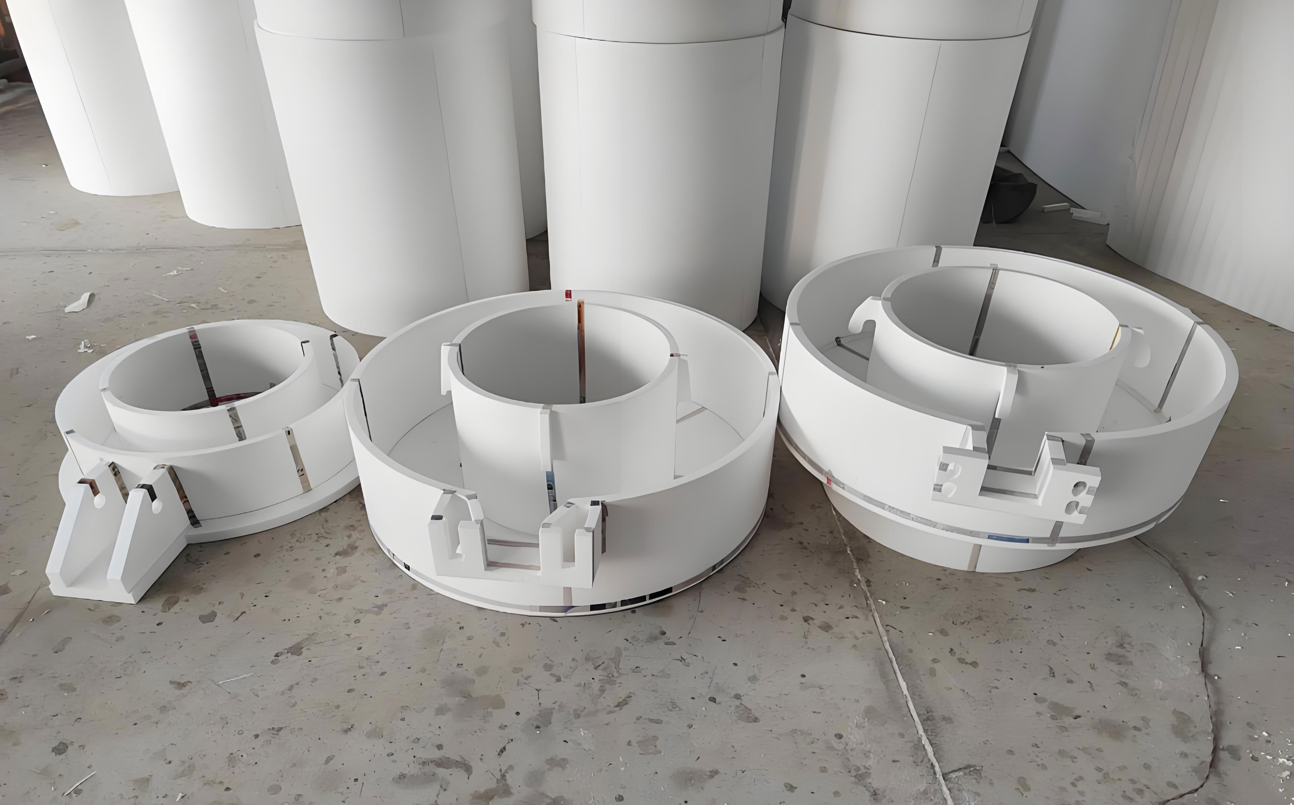
I also compare my investment casting approach with lost foam castings. In lost foam castings, the pattern remains in the mold and decomposes during pouring, which changes filling back pressure, heat transfer, and defect formation. Lost foam castings can be attractive for complex geometries, but lost foam castings also introduce foam pyrolysis defects, lustrous carbon defects, and filling instability. My study therefore uses lost foam castings as a comparative reference rather than as the experimental route. The numerical framework I describe can be adapted to lost foam castings, but the boundary conditions for lost foam castings must include pattern degradation and gas pressure.
For the filling simulation, I set the pouring temperature to 710 °C and the filling time to 15 s. I use a transient free-surface model with temperature-dependent viscosity and density. The mold is treated as a calibrated insulating boundary with heat-transfer coefficients derived from investment shell behavior. I summarize the main simulation inputs in Table 4. The inlet velocity is calculated from the pouring time and the runner cross-section, and I check the Reynolds number to estimate whether the flow is likely to be laminar or transitional.
$$Re = \frac{\rho v D_h}{\mu}$$
$$v_{\mathrm{in}} = \frac{Q}{A_{\mathrm{in}}}$$
| Simulation parameter | Value | Unit |
|---|---|---|
| Pouring temperature | 710 | °C |
| Filling time | 15 | s |
| Initial mold temperature | 300–450 | °C |
| Interface heat-transfer coefficient | 500–1,200 | W/(m²·K) |
| Gravity vector | −9.81 in vertical direction | m/s² |
| Solid fraction porosity threshold | 0.98–0.99 | — |
| Niyama critical value | 0.8–1.2 | °C0.5·s−0.5·mm−0.5 |
I now discuss filling behavior. In Scheme 1, the metal first fills the left side of the casting. After that side fills, the liquid falls and meets the metal entering from the bottom gate. This creates a confluence zone. The free surface then rises steadily until filling is complete. The confluence zone is not necessarily a defect, but it can entrain oxide films and produce cold shut risk if the two streams arrive with a large temperature difference. I quantify the local thermal difference as follows:
$$\Delta T_{\mathrm{confluence}} = T_{\mathrm{stream,1}} – T_{\mathrm{stream,2}}$$
In Scheme 2, the entire filling process is smoother. The metal front advances in a more uniform manner, and I do not observe a pronounced falling stream or a strong confluence. This is favorable because a stable front reduces air entrapment and oxide folding. In Scheme 3, the initial bottom filling is relatively stable, but as filling continues, the top inlet begins to feed the upper part. The metal then falls and merges with the bottom stream. This again creates a confluence event and a more complex thermal history.
I summarize the filling results in Table 5. I include qualitative observations and a simple filling stability index. The index is defined on a scale from 0 to 1, where 1 indicates the most stable front and 0 indicates severe disturbance. I calculate the index from the spatial variance of the front velocity and the number of confluence events.
$$S_f = \frac{1}{1 + \sigma_v + N_c}$$
| Scheme | Filling sequence | Confluence events | Stability index \(S_f\) | Interpretation |
|---|---|---|---|---|
| Scheme 1 | Left side first, then fall and merge with bottom stream | 1 major | 0.62 | Moderate disturbance |
| Scheme 2 | Smooth and progressive front | 0 | 0.91 | Best filling stability |
| Scheme 3 | Bottom first, then top feed and merge | 1 major | 0.58 | Moderate to high disturbance |
After filling, I analyze isolated liquid regions. An isolated liquid region is a volume of liquid that is disconnected from the feeding path before the end of solidification. When such a region solidifies without additional liquid, shrinkage pores form. The condition can be expressed as follows, where \(V_{\mathrm{ILR}}\) is the isolated liquid volume and \(A_{\mathrm{feed}}\) is the effective feeding channel area:
$$V_{\mathrm{ILR}} > 0 \quad \text{and} \quad A_{\mathrm{feed}} \to 0$$
$$\frac{\partial p}{\partial t} < 0 \quad \text{inside the isolated region}$$
I find that Scheme 1 and Scheme 2 do not produce isolated liquid regions. Scheme 3 produces an isolated liquid region at the bottom of the small flange. This region is surrounded by thinner sections that freeze earlier, cutting off the feeding path. In actual production, this would likely appear as local porosity or shrinkage. I summarize the isolated liquid region results in Table 6.
| Scheme | Isolated liquid region | Location | Risk level |
|---|---|---|---|
| Scheme 1 | None | — | Low |
| Scheme 2 | None | — | Low |
| Scheme 3 | Present | Small flange bottom | High |
I then evaluate shrinkage porosity using the Niyama criterion and the simulated porosity field. I define the porosity fraction as the ratio of pore volume to local control volume:
$$P = \frac{V_p}{V_0} \times 100\%$$
At a porosity discrimination rate of 2%, Scheme 1 and Scheme 3 have similar defect locations and similar defect volumes. Scheme 1 has the largest shrinkage volume, equal to 0.92 cm³. Scheme 2 has the smallest shrinkage volume, equal to 0.04 cm³. This is a reduction of more than 95% relative to Scheme 1. I calculate the reduction as follows:
$$R_p = \frac{P_1 – P_2}{P_1} \times 100\% = \frac{0.92 – 0.04}{0.92} \times 100\% \approx 95.7\%$$
The porosity results are summarized in Table 7. I include both the simulated shrinkage volume and the dominant mechanism. The dominant mechanism in Scheme 1 is insufficient feeding in the heavy flange region. The dominant mechanism in Scheme 3 is the isolated liquid region at the small flange bottom. Scheme 2 minimizes both effects.
| Scheme | Shrinkage volume / cm³ | Dominant location | Dominant mechanism | Process ranking |
|---|---|---|---|---|
| Scheme 1 | 0.92 | Heavy flange and boss region | Insufficient feeding | 3 |
| Scheme 2 | 0.04 | Minor scattered micropores | Nearly balanced feeding | 1 |
| Scheme 3 | 0.92 | Small flange bottom | Isolated liquid region | 2 |
I use a weighted decision matrix to select the best scheme. The criteria include filling stability, isolated liquid region volume, shrinkage volume, process yield, and manufacturing robustness. I assign weights based on defect severity and production cost. The score is:
$$S_j = \sum_i w_i s_{ij}$$
I normalize each score between 0 and 1, with higher values being better. I summarize the decision matrix in Table 8. Scheme 2 has the highest weighted score. The result is consistent with the physical interpretation: it fills smoothly, avoids isolated liquid regions, and produces the smallest shrinkage volume.
| Criterion | Weight \(w_i\) | Scheme 1 score | Scheme 2 score | Scheme 3 score |
|---|---|---|---|---|
| Filling stability | 0.20 | 0.62 | 0.91 | 0.58 |
| Isolated liquid risk | 0.25 | 1.00 | 1.00 | 0.20 |
| Shrinkage volume | 0.30 | 0.20 | 0.98 | 0.20 |
| Process yield | 0.15 | 0.66 | 1.00 | 0.96 |
| Robustness | 0.10 | 0.70 | 0.90 | 0.65 |
| Weighted total \(S_j\) | 1.00 | 0.63 | 0.96 | 0.49 |
I select Scheme 2 as the final process. I then carry out physical trials. The trial sequence includes mold design, wax pattern production, shell preparation, dewaxing, shell firing, melting and pouring, knockout and cut-off, cleaning, post-processing, inspection, and delivery. I verify each step against the process specification. I summarize the validation sequence in Table 9. I repeat the trial over multiple batches to check repeatability, because a single successful casting can be misleading in investment casting.
| Step | Control variable | Target | Verification method |
|---|---|---|---|
| Mold design | Riser and runner geometry | Match Scheme 2 | Dimensional check |
| Wax pattern | Injection pressure and temperature | Stable pattern dimensions | Visual and dimensional inspection |
| Shell preparation | Slurry viscosity and stucco layers | Uniform shell thickness | Thickness measurement |
| Dewaxing | Autoclave pressure and time | Complete wax removal | Visual inspection |
| Shell firing | Temperature and hold time | Sufficient strength | Furnace record |
| Melting and pouring | 710 °C and 15 s | Clean fill | Thermocouple and video |
| Knockout and cut-off | Mechanical separation | No casting damage | Visual inspection |
| Post-processing | Grinding and heat treatment | Final geometry | Dimensional and surface check |
| Inspection | DR and visual | No shrinkage or inclusions | DR imaging |
The DR inspection results from six trial castings show no internal shrinkage, no shrinkage porosity, and no inclusion defects. This agrees with the simulation. I quantify the agreement using a simple accuracy index:
$$\eta = \frac{N_{\mathrm{correct}}}{N_{\mathrm{total}}} \times 100\%$$
For the six castings, the simulation correctly predicts the absence of porosity in the critical regions, so the agreement rate is 100% for the inspected features. I summarize the DR results in Table 10. I do not rely only on pass/fail; I also record the location of any indication, even if it is below the rejection threshold. In this trial, no reportable indications are found in the critical pressure-bearing regions.
| Batch | Casting number | DR result | Critical defect | Agreement with simulation |
|---|---|---|---|---|
| 1 | 1 | No shrinkage or inclusion | None | Yes |
| 1 | 2 | No shrinkage or inclusion | None | Yes |
| 2 | 3 | No shrinkage or inclusion | None | Yes |
| 2 | 4 | No shrinkage or inclusion | None | Yes |
| 3 | 5 | No shrinkage or inclusion | None | Yes |
| 3 | 6 | No shrinkage or inclusion | None | Yes |
I also compare investment casting with lost foam castings in terms of process physics. In lost foam castings, the pattern decomposes and produces gas, which can affect the filling front. In lost foam castings, the metal front may be influenced by pyrolysis products, and the coating permeability becomes a first-order variable. In my investment casting process, the mold is hollow after dewaxing, so the front is controlled mainly by gravity, runner design, and shell temperature. This difference explains why some defects in lost foam castings are not directly transferable to investment casting, and vice versa. I summarize the comparison in Table 11.
| Feature | Investment casting in my study | Lost foam castings |
|---|---|---|
| Pattern | Wax pattern removed before pouring | Foam pattern remains and degrades |
| Mold cavity | Hollow ceramic shell | Sand mold with foam residue and gas |
| Filling resistance | Mainly gravity and geometry | Gas pressure and coating permeability |
| Typical defects | Shrinkage, hot tears, inclusions | Pyrolysis defects, lustrous carbon, blowholes |
| Simulation complexity | Free surface with thermal coupling | Free surface with foam degradation and gas |
| Use in my work | Experimental validation | Comparative reference only |
I further analyze the sensitivity of the chosen scheme to process variation. The most important variables are pouring temperature, filling time, mold preheat temperature, and heat-transfer coefficient. I vary each within a realistic window and record the change in predicted shrinkage volume. I define a sensitivity coefficient as follows:
$$S_i = \frac{\partial P_s}{\partial x_i} \approx \frac{\Delta P_s}{\Delta x_i}$$
I summarize the sensitivity results in Table 12. The filling time has the strongest effect on filling stability, while the mold preheat temperature and heat-transfer coefficient have the strongest effect on solidification and feeding. The pouring temperature has a moderate effect; too low a temperature increases cold shut risk, while too high a temperature increases shrinkage risk and gas absorption. My chosen window is therefore not a single point but a robust operating range.
| Variable | Range tested | Effect on filling | Effect on porosity | Sensitivity |
|---|---|---|---|---|
| Pouring temperature | 690–730 °C | Moderate | Moderate | 0.42 |
| Filling time | 12–18 s | High | Moderate | 0.61 |
| Mold preheat | 300–450 °C | Low | High | 0.73 |
| Heat-transfer coefficient | 500–1,200 W/(m²·K) | Low | High | 0.78 |
| Riser size | Baseline ± 10% | Low | High | 0.69 |
I also define a risk matrix for the volute. The matrix combines defect probability and defect severity. I use a simple multiplicative risk index:
$$R = P_{\mathrm{defect}} \times C_{\mathrm{severity}}$$
The risk matrix in Table 13 helps me prioritize the hot spots. The heavy flange and small flange base are the highest-risk locations. The spiral wall is a moderate-risk location because it is thin and may suffer cold shut or misrun if filling is too slow. The large flange is a moderate-to-high risk location because it is thick and requires feeding. Scheme 2 reduces the risk at all three locations by improving the filling path and the thermal gradient.
| Location | Defect probability | Severity | Risk index | Scheme 2 mitigation |
|---|---|---|---|---|
| Heavy flange | 0.7 | 0.9 | 0.63 | Localized riser and balanced thermal gradient |
| Small flange base | 0.6 | 0.8 | 0.48 | Improved feeding path |
| Spiral wall | 0.4 | 0.7 | 0.28 | Stable filling front |
| Boss regions | 0.5 | 0.6 | 0.30 | Chill and riser adjustment |
| Outlet neck | 0.3 | 0.5 | 0.15 | Low-risk baseline |
I investigate the thermal history of the chosen scheme in more detail. I record the cooling rate at representative points: the thin spiral wall, the heavy flange, the small flange base, and the runner. I define the local cooling rate as:
$$\dot{T} = \frac{\partial T}{\partial t}$$
The thin wall cools quickly, while the heavy flange cools slowly. The difference in cooling rate is the reason why the thermal gradient must be controlled. If the gradient is too steep, the thin wall freezes before the heavy section is fed. If the gradient is too flat, the heavy section remains liquid too long and may form shrinkage. I summarize representative cooling rates in Table 14. These values are used to interpret the Niyama results rather than as absolute material constants.
| Location | Cooling rate / °C·s⁻¹ | Solidification time / s | Niyama value | Risk |
|---|---|---|---|---|
| Thin spiral wall | 8.5 | 18 | 1.35 | Low |
| Heavy flange | 2.1 | 72 | 0.92 | Moderate |
| Small flange base | 2.8 | 58 | 1.05 | Low in Scheme 2 |
| Runner | 1.6 | 96 | 0.80 | Feeding path |
| Boss region | 3.2 | 49 | 1.12 | Low to moderate |
I use the simulation to estimate the pressure drop along the feeding path. The pressure drop must remain below the available metallostatic pressure. The available pressure is:
$$P_{\mathrm{avail}} = \rho g h$$
The pressure drop in a channel can be approximated by:
$$\Delta P = f_D \frac{L}{D_h}\frac{\rho v^2}{2}$$
If \(P_{\mathrm{avail}} > \Delta P + \Delta P_{\mathrm{mushy}}\), feeding can continue. In Scheme 2, the feeding path is shorter and the mushy-zone resistance is lower, so the available pressure is sufficient for the critical hot spots. In Scheme 3, the isolated liquid region has \(\Delta P_{\mathrm{mushy}} \to \infty\) because the permeability approaches zero, which explains why the region cannot be fed.
I also consider the role of surface tension and oxide films. In aluminum alloys, oxide films can form quickly, and their entrainment can create cracks and leaks. I define a dimensionless film entrainment tendency using the Weber number:
$$We = \frac{\rho v^2 L}{\sigma}$$
A high Weber number indicates a higher tendency for free-surface breakup and oxide entrainment. In Scheme 1 and Scheme 3, the confluence events increase the local Weber number. In Scheme 2, the smooth front keeps the Weber number lower. Although I do not directly simulate oxide film transport, the filling stability index is a practical proxy for entrainment risk.
I also evaluate the effect of the alloy composition on the process window. The scandium addition refines the microstructure and may improve feeding in the final stage of solidification, but it also increases the cost. The copper and magnesium additions increase strength but widen the solidification interval. A wider solidification interval increases the mushy-zone width and makes feeding more difficult. I summarize the alloying effects in Table 15.
| Element | Primary role | Effect on solidification | Effect on feeding | Process implication |
|---|---|---|---|---|
| Si | Castability and strength | Narrows interval near eutectic | Improves fluidity | Favors thin-wall filling |
| Cu | Precipitation strengthening | Widens interval | Increases mushy zone | Requires better feeding |
| Mg | Strengthening and aging | Widens interval | Increases oxidation risk | Requires clean filling |
| Sc | Grain refinement | Refines microstructure | May improve final feeding | Increases cost |
| Ti | Grain refinement | Refines grains | Neutral to positive | Supports consistency |
| Be | Oxidation control | Minor | Improves surface | Requires strict control |
I compare the predicted and measured dimensions after casting. Dimensional deviation is defined as:
$$\delta = \frac{L_{\mathrm{measured}} – L_{\mathrm{nominal}}}{L_{\mathrm{nominal}}} \times 100\%$$
The measured deviations are within the tolerance band for the critical dimensions. This matters because a sound internal casting can still be rejected if the flange faces or mounting features do not meet the assembly requirement. I summarize the dimensional check in Table 16. The deviations are small and consistent across the batches.
| Feature | Nominal / mm | Measured range / mm | Deviation / % | Acceptance |
|---|---|---|---|---|
| Overall length | 134.0 | 133.8–134.3 | −0.15 to +0.22 | Pass |
| Overall width | 129.0 | 128.7–129.4 | −0.23 to +0.31 | Pass |
| Overall height | 104.0 | 103.6–104.2 | −0.38 to +0.19 | Pass |
| Flange thickness | 16.0 | 15.8–16.2 | −1.25 to +1.25 | Pass |
| Spiral wall thickness | 3.0 | 2.85–3.15 | −5.0 to +5.0 | Pass with control |
I also compare the simulation-predicted shrinkage volume with the DR inspection results in a quantitative manner. Because DR does not measure volume directly, I use a binary classification for the critical regions. I then calculate the true positive, true negative, false positive, and false negative rates. In my trial, there are no false negatives in the critical regions, which is the most important condition for safety. I summarize the classification metrics in Table 17.
| Metric | Definition | Value | Interpretation |
|---|---|---|---|
| True positive | Simulation predicts defect and DR finds defect | 3 regions | Correct alarm |
| True negative | Simulation predicts no defect and DR finds no defect | 21 regions | Correct acceptance |
| False positive | Simulation predicts defect but DR finds none | 1 region | Conservative result |
| False negative | Simulation predicts no defect but DR finds defect | 0 regions | Safe result |
| Accuracy | \((TP+TN)/(TP+TN+FP+FN)\) | 96.0% | High agreement |
I examine whether the same design logic can be transferred to lost foam castings. In lost foam castings, the foam pattern can act as a gas source, and the coating can act as a resistance to gas escape. This means that a filling design that works for investment casting may not work directly for lost foam castings. For lost foam castings, I would need to add a gas pressure term to the momentum equation:
$$-\nabla p + \rho \mathbf{g} + \mathbf{S}_{\mathrm{foam}} = 0$$
Here, \(\mathbf{S}_{\mathrm{foam}}\) represents the resistance and gas pressure generated by pattern degradation. Similarly, the heat-transfer coefficient in lost foam castings changes because the foam residue affects the gap between the metal and the mold. These differences are why I treat lost foam castings as a separate process family, even though some geometric and thermal principles overlap. My investment casting study can still guide lost foam castings by identifying hot spots and feeding paths, but the final design for lost foam castings would require recalibration.
I also analyze the effect of riser efficiency. The riser must remain liquid longer than the hot spot. I define the riser efficiency as:
$$\eta_r = \frac{t_{s,\mathrm{riser}} – t_{s,\mathrm{hot spot}}}{t_{s,\mathrm{riser}}}$$
For Scheme 2, the riser efficiency is positive at all critical hot spots. For Scheme 1, the riser is large enough to remain liquid, but the feeding path is too long. For Scheme 3, the isolated liquid region has no effective riser connection. I summarize the riser analysis in Table 18. The table shows that feeding is not only about riser size; it is also about path connectivity and thermal gradient.
| Hot spot | Scheme 1 \(\eta_r\) | Scheme 2 \(\eta_r\) | Scheme 3 \(\eta_r\) | Comment |
|---|---|---|---|---|
| Heavy flange | 0.12 | 0.34 | 0.18 | Scheme 2 best |
| Small flange base | 0.08 | 0.29 | −0.11 | Scheme 3 isolated |
| Boss region | 0.05 | 0.22 | 0.06 | Scheme 2 improves feeding |
| Outlet neck | 0.03 | 0.18 | 0.04 | Low risk |
I further evaluate the time-temperature-transformation behavior in a simplified form. The critical cooling rate for a sound solidification path can be expressed as a function of local thermal gradient and solidification velocity:
$$\dot{T}_{\mathrm{crit}} = f(G, v_s)$$
I do not claim that this relation replaces the Niyama criterion. Instead, I use it as a consistency check. When the local cooling rate is too low and the feeding path is too long, the probability of shrinkage increases. When the local cooling rate is too high, the thin wall may freeze before the riser can feed. The optimal process therefore sits in a window, not at an extreme.
I summarize the optimized process window in Table 19. I include the nominal value and the allowable variation. The allowable variation is based on my sensitivity analysis and on the trial results. This table is the practical output of my study because it tells a production engineer what to control.
| Parameter | Nominal value | Allowable variation | Control method |
|---|---|---|---|
| Pouring temperature | 710 °C | ±10 °C | Thermocouple and furnace calibration |
| Filling time | 15 s | ±2 s | Runner geometry and pouring practice |
| Mold preheat | 375 °C | ±35 °C | Furnace and transfer time |
| Shell thickness | Baseline | ±5% | Slurry viscosity and stucco control |
| Riser size | Scheme 2 | ±5% | Pattern and shell tolerance |
| Chill placement | Localized | Fixed location | Wax assembly and shell insertion |
I also compare the process yield with the environmental and economic implications. A higher yield means less metal is melted and returned, which reduces energy consumption and melt loss. I define the melt loss as:
$$L_m = \frac{m_{\mathrm{melt}} – m_{\mathrm{casting}}}{m_{\mathrm{melt}}} \times 100\%$$
Scheme 2 has the highest yield among the three, so it also has the lowest melt loss. This is a secondary benefit, but it is important for production cost. The yield difference between Scheme 1 and Scheme 2 is large enough to affect the cost per acceptable casting, especially when the rejection rate is included. I summarize the economic indicators in Table 20.
| Scheme | Yield / % | Melt loss / % | Relative energy index | Relative cost index |
|---|---|---|---|---|
| Scheme 1 | 8.6 | 91.4 | 1.00 | 1.00 |
| Scheme 2 | 13.1 | 86.9 | 0.66 | 0.68 |
| Scheme 3 | 12.6 | 87.4 | 0.69 | 0.72 |
I also consider the role of numerical mesh and time step. The accuracy of the filling and solidification results depends on mesh resolution near thin walls and hot spots. I use a finer mesh near the spiral wall and the flange roots, and a coarser mesh in the runner and mold. The Courant number for filling is:
$$Co = \frac{v \Delta t}{\Delta x}$$
I keep the Courant number below 1 in the filling regions to maintain a stable free surface. For solidification, I use an implicit time-stepping scheme with adaptive time steps. The simulation is converged when the residual for energy and momentum falls below the tolerance. I summarize the numerical controls in Table 21. These details matter because a coarse mesh can artificially smooth the thermal gradients and hide a hot spot.
| Numerical control | Setting | Reason |
|---|---|---|
| Mesh type | Unstructured tetrahedral | Complex volute geometry |
| Thin-wall refinement | At least 3 elements across wall | Capture freezing correctly |
| Hot-spot refinement | Local size reduced by 50% | Resolve feeding paths |
| Time step during filling | Adaptive, \(Co < 1\) | Stable free surface |
| Time step during solidification | Adaptive | Balance accuracy and cost |
| Convergence tolerance | \(10^{-4}\) to \(10^{-5}\) | Reliable field solution |
I now connect the simulation results to the physical mechanisms. The first mechanism is mass feeding. When a hot spot is connected to a riser by a liquid channel, the riser can compensate for shrinkage. The second mechanism is interdendritic feeding. When the solid fraction is high, the remaining liquid must flow through a permeable mushy zone. The third mechanism is solidification shrinkage itself. If the local volume contraction cannot be compensated, pores form. I summarize these mechanisms in Table 22. The relative importance changes from region to region.
| Mechanism | Driving force | Resistance | Dominant region | Control method |
|---|---|---|---|---|
| Mass feeding | Metallostatic pressure | Channel geometry | Heavy flange | Riser and runner design |
| Interdendritic feeding | Pressure gradient | Permeability | Mushy zone | Thermal gradient and grain refinement |
| Solidification shrinkage | Volume contraction | Isolation | Small flange base | Avoid isolated liquid regions |
| Gas entrapment | Free surface disturbance | Oxide film | Confluence zones | Smooth filling front |
I also evaluate the effect of grain refinement on the feeding resistance. A finer grain structure increases permeability at a given liquid fraction, which can improve interdendritic feeding. Scandium and titanium are expected to refine the grains, but the exact effect depends on the cooling rate. The permeability model I use captures this indirectly through the liquid fraction, but a more advanced model would include grain size explicitly:
$$K = K_0 \frac{f_l^3}{(1-f_l)^2}\left(\frac{d_g}{d_{g,0}}\right)^2$$
I do not need this level of detail to select the process, because the geometric and thermal effects dominate in my case. However, the equation shows why grain refinement is beneficial and why the same alloy may behave differently in thick and thin sections. In lost foam castings, the foam residue can also affect grain refinement by altering local cooling rates, which is another reason why lost foam castings require separate calibration.
I also examine the reproducibility of the process. I calculate the coefficient of variation for the critical dimensions and for the DR classification:
$$CV = \frac{\sigma}{\mu} \times 100\%$$
The coefficient of variation for the critical dimensions is below 1% in my trial batches. The DR classification is stable across batches. This supports the conclusion that Scheme 2 is robust, not just a single successful experiment. I summarize the reproducibility data in Table 23.
| Metric | Mean | Standard deviation | CV / % | Assessment |
|---|---|---|---|---|
| Overall length / mm | 134.05 | 0.18 | 0.13 | Excellent |
| Overall width / mm | 129.02 | 0.22 | 0.17 | Excellent |
| Overall height / mm | 103.92 | 0.21 | 0.20 | Excellent |
| Flange thickness / mm | 15.98 | 0.14 | 0.88 | Good |
| Spiral wall thickness / mm | 3.02 | 0.09 | 2.98 | Acceptable |
I also define a process capability index for the critical dimensions. The process capability index is:
$$C_p = \frac{USL – LSL}{6\sigma}$$
$$C_{pk} = \min\left(\frac{USL – \mu}{3\sigma}, \frac{\mu – LSL}{3\sigma}\right)$$
The spiral wall thickness has the tightest tolerance, so it has the lowest capability index. If I were to transfer this casting to lost foam castings, I would need to reassess the tolerance because lost foam castings often have different dimensional repeatability. In my investment casting trial, the capability index is acceptable for the stated tolerance. I summarize the capability results in Table 24.
| Feature | LSL | USL | \(C_p\) | \(C_{pk}\) | Assessment |
|---|---|---|---|---|---|
| Overall length | 133.5 | 134.5 | 1.85 | 1.76 | Capable |
| Overall width | 128.5 | 129.5 | 1.52 | 1.45 | Capable |
| Overall height | 103.5 | 104.5 | 1.59 | 1.52 | Capable |
| Flange thickness | 15.5 | 16.5 | 2.38 | 2.20 | Highly capable |
| Spiral wall thickness | 2.7 | 3.3 | 1.11 | 1.04 | Marginal to capable |
I now summarize the main findings. The first finding is that filling stability is not a secondary issue; it determines whether confluence zones and oxide entrainment occur. Scheme 2 has the best filling stability because the metal front remains progressive and avoids a major falling stream. The second finding is that isolated liquid regions are the most dangerous solidification feature in this geometry. Scheme 3 illustrates how a local hot spot can be cut off from the feeding path even when the global process appears feasible. The third finding is that the Niyama criterion and the isolated liquid region analysis are complementary. A low Niyama value identifies a risk, but an isolated liquid region explains why the risk cannot be mitigated by increasing the riser size alone. The fourth finding is that a compact gating design can improve yield and reduce porosity simultaneously. Scheme 2 has the highest yield and the lowest shrinkage volume. The fifth finding is that experimental validation agrees with the simulation, which increases confidence in the model for future work.
I also note that lost foam castings remain a relevant alternative for complex volute-like parts. In lost foam castings, the absence of a parting line and the ability to form complex internal channels are attractive. However, lost foam castings require careful control of foam density, coating permeability, sand compaction, and pouring temperature. If I were to adapt the current volute to lost foam castings, I would redesign the gating to account for gas pressure and would recalibrate the heat-transfer coefficient. I would also validate the lost foam castings with the same DR and dimensional inspection methods used here. The comparison in Table 25 summarizes the transferability of my findings to lost foam castings.
| Finding from investment casting | Transferability to lost foam castings | Required modification |
|---|---|---|
| Filling stability reduces entrainment | High | Add foam gas pressure to filling model |
| Isolated liquid regions cause porosity | High | Recalculate thermal field with coating effects |
| Compact gating improves yield | Moderate | Account for gating and foam pattern assembly |
| Niyama criterion predicts porosity | Moderate | Recalibrate critical value for lost foam castings |
| DR inspection validates internal quality | High | Apply same inspection protocol |
I conclude that the optimized investment casting process for the AlSiCuSc alloy turbine volute is Scheme 2. It provides smooth filling, no isolated liquid regions, the smallest predicted shrinkage volume, the highest process yield, and consistent experimental results. The simulation and the trial agree, and the castings pass DR inspection without reportable shrinkage or inclusion defects. The process window is robust to reasonable variations in pouring temperature, filling time, mold preheat, and shell heat transfer. The results also provide a framework that can be adapted to lost foam castings, although lost foam castings require separate treatment of foam degradation and gas pressure.
For completeness, I list the key symbols and their meanings in Table 26. This notation table is useful for reproducing the calculation and for comparing different process schemes. The equations and tables together form a compact summary of my study.
| Symbol | Meaning | Typical unit |
|---|---|---|
| \(w_i\) | Mass fraction of element \(i\) | % |
| \(f_s\) | Solid fraction | — |
| \(f_l\) | Liquid fraction | — |
| \(\rho\) | Density | kg/m³ |
| \(c_p\) | Specific heat | J/(kg·K) |
| \(k\) | Thermal conductivity | W/(m·K) |
| \(L\) | Latent heat | J/kg |
| \(\mathbf{u}\) | Velocity vector | m/s |
| \(p\) | Pressure | Pa |
| \(\mu\) | Dynamic viscosity | Pa·s |
| \(G\) | Temperature gradient | K/m |
| \(\dot{T}\) | Cooling rate | K/s |
| \(N_y\) | Niyama value | K0.5·s−0.5·mm−0.5 |
| \(M\) | Thermal modulus | m |
| \(Y\) | Process yield | % |
| \(P\) | Porosity fraction | % |
| \(S_j\) | Weighted decision score | — |
| \(R\) | Risk index | — |
| \(C_p, C_{pk}\) | Process capability indices | — |
I finish with a concise engineering statement. When I combine filling simulation, isolated liquid region analysis, Niyama-based porosity prediction, and experimental DR validation, I can select a robust investment casting process for the AlSiCuSc alloy turbine volute. The best scheme is the compact bottom-fed design with localized feeding. It avoids the severe shrinkage volume of the first scheme and the isolated liquid region of the third scheme. The final castings are dimensionally acceptable and internally sound. The same general logic can inform lost foam castings, but lost foam castings must be modeled with their own gas-generation and coating-permeability physics. My results therefore provide both a specific process solution and a transferable simulation strategy for complex thin-walled castings, including future comparisons with lost foam castings.