
In modern manufacturing, the quality of precision castings is of paramount importance, especially for components used in automotive, aerospace, and heavy machinery industries. Among various manufacturing defects, surface cracks and internal flaws can significantly reduce the service life and safety of mechanical parts. Magnetic particle inspection (MPI) is commonly employed to detect surface and near-surface defects in ferromagnetic materials. However, traditional MPI heavily relies on human inspectors, which introduces subjective bias, fatigue-related errors, and limited throughput. To overcome these limitations, I have developed an automatic defect detection system for precision castings using deep convolutional neural networks (CNNs). This thesis focuses on the research and application of deep learning methods for detecting sand foundry defects in precision castings, with an emphasis on achieving high accuracy, low false-negative rate, and real-time performance through embedded system deployment.
The core contribution of this work is a systematic study of network architecture optimization for classifying magnetic particle images of castings into defective and non-defective categories. I first constructed a deep learning environment based on GPU acceleration and the Caffe framework. Then I investigated the effects of hyperparameters, convolution kernel sizes, network depth, and pooling strategies on model performance. By tuning these parameters and simplifying the network structure, I achieved a training accuracy of 99% on the validation set. Finally, I ported the trained CNN model to an NVIDIA Jetson TX1 embedded platform, where the system achieved a final accuracy of 98.67% on a test set of 600 images, with zero missed defects. The embedded system meets industrial requirements for speed and reliability, demonstrating the practical viability of deep learning for sand foundry defects inspection.
This chapter begins with a review of the background and significance of defect detection, followed by an overview of deep learning research, and then details the methodology, experiments, and embedded implementation. Throughout the paper, I emphasize the importance of adapting network architectures to the specific characteristics of sand foundry defects, such as small crack sizes, complex backgrounds, and variable lighting conditions in magnetic particle images.
1. Introduction
The manufacturing industry has experienced rapid growth in recent years, particularly in the production of complex mechanical components. Precision castings, such as engine blocks, gear housings, and hydraulic valve bodies, are susceptible to various defects during the casting process. These defects include cracks, porosity, shrinkage cavities, and inclusions. According to statistical data, fatigue failure accounts for approximately 80% of mechanical component failures, and most fatigue cracks originate from surface defects. Therefore, timely and accurate detection of surface flaws is critical to ensuring product quality and operational safety.
Non-destructive testing (NDT) methods are widely used for defect detection without damaging the inspected part. Among them, magnetic particle testing is especially effective for ferromagnetic materials due to its high sensitivity, simplicity, and low cost. In magnetic particle testing, the workpiece is magnetized, and ferrous particles are applied to the surface. A crack or flaw creates a leakage magnetic field that attracts the particles, forming a visible indication. However, the interpretation of magnetic particle images is traditionally performed by trained inspectors, which is labor-intensive and prone to human error. To address these issues, researchers have explored automated image processing techniques, but conventional algorithms often struggle with the variability of defect shapes and complex backgrounds.
Deep learning has emerged as a powerful tool for image classification and object detection. Convolutional neural networks (CNNs) can automatically learn hierarchical features from raw images, eliminating the need for manually engineered features. Since the groundbreaking success of AlexNet in the ImageNet competition, deep CNNs have been widely applied in various fields, including medical imaging, remote sensing, and industrial inspection. For sand foundry defects, deep learning offers the potential to achieve higher detection accuracy and speed compared to traditional machine vision methods.
In this thesis, I focus on the detection of cracks in precision castings using magnetic particle images. The main objectives are:
- To construct a deep learning training environment using GPU and Caffe.
- To design and optimize a CNN architecture for the specific characteristics of sand foundry defects.
- To investigate the impact of kernel size, network depth, hyperparameters, and pooling methods on model accuracy and training efficiency.
- To deploy the trained model on an embedded platform (Jetson TX1) and evaluate its real-world performance.
The rest of this paper is organized as follows. Section 2 describes the deep learning environment, including hardware and software selection, and introduces the basic CNN components. Section 3 details the application of deep learning to magnetic particle defect detection, including sample preparation, network architecture design, and experimental optimization. Section 4 presents the embedded system implementation and performance evaluation. Finally, Section 5 summarizes the work and outlines future directions.
2. Deep Learning Environment Construction
2.1 Hardware Platform Selection
Deep learning models require large amounts of data and intensive computation. Training a CNN on millions of parameters involves massive matrix operations that are more efficiently executed on graphics processing units (GPUs) than on central processing units (CPUs). The architectures of GPUs and CPUs are fundamentally different. As shown in Figure 2.1 (conceptual diagram), GPUs contain many arithmetic logic units (ALUs) that perform parallel computations, whereas CPUs have a smaller number of ALUs but more sophisticated control and cache units. Because neural network training is data-parallel, GPUs can accelerate the training process by several orders of magnitude.
For this research, I selected the NVIDIA GeForce GTX 1080 GPU. This GPU has 2560 CUDA cores, a base clock of 1607 MHz, a boost clock of 1733 MHz, and 8 GB of GDDR5X memory. Its single-precision floating-point performance reaches 9 Teraflops, which is sufficient for training moderate-sized CNNs. The primary parameters of the GTX 1080 are summarized in the table below.
| Parameter | Value |
|---|---|
| CUDA Cores | 2560 |
| Base Clock | 1607 MHz |
| Boost Clock | 1733 MHz |
| Memory | 8 GB GDDR5X |
| Memory Bandwidth | 320 GB/s |
| Power Consumption | 180 W |
2.2 Software Platform Selection
I chose Caffe (Convolutional Architecture for Fast Feature Embedding) as the deep learning framework. Caffe is an open-source library that provides a clean and modifiable framework for implementing deep learning algorithms. Its advantages include:
- Fast: Caffe is optimized for GPU acceleration and can process large datasets efficiently.
- Modular: Network architectures are defined in configuration files (e.g., .prototxt), making it easy to modify layers and parameters without writing code.
- Openness: Pretrained models and network definitions are publicly available, which accelerates development.
- Community: A large user community provides support and continuous improvements.
The Caffe environment was installed on Ubuntu 14.04. Key dependencies include:
- gcc/g++ compiler suite
- Protobuf (Protocol Buffers) for data serialization
- Boost libraries for C++ extensions
- GFlags for command-line argument parsing
- GLog for logging training information
- BLAS (Basic Linear Algebra Subprograms) for linear algebra operations
- HDF5 for hierarchical data storage
- OpenCL for heterogeneous computing
- LMDB/LEVELDB for database management
- Python bindings for scripting
2.3 Convolutional Neural Network Fundamentals
A CNN is composed of multiple layers, including convolutional layers, pooling layers, activation layers, fully connected layers, and loss layers. The operation of a convolutional layer can be expressed as:
$$ X_j^l = f\left( \sum_{i \in M_j} X_i^{l-1} * K_{ij}^l + b_j^l \right) $$
where $X_j^l$ is the $j$-th feature map at layer $l$, $M_j$ is the set of input feature maps, $K_{ij}^l$ is the convolution kernel between input $i$ and output $j$, $b_j^l$ is the bias term, and $f(\cdot)$ is the activation function. The output feature map size is computed by:
$$ w_1 = \frac{w_0 + 2 \times pad – kernel\_size}{stride} + 1 $$
$$ h_1 = \frac{h_0 + 2 \times pad – kernel\_size}{stride} + 1 $$
Pooling layers down-sample feature maps to reduce computational load and provide spatial invariance. Common pooling operations include max pooling and average pooling, defined respectively as:
$$ P_n = \max_{i \in R_n} C_i $$
$$ P_n = \frac{1}{|R_n|} \sum_{i \in R_n} C_i $$
Activation functions introduce non-linearity. Popular choices are Sigmoid, Tanh, and ReLU. ReLU is often preferred because it accelerates convergence:
$$ \mathrm{ReLU}(x) = \max(0, x) $$
2.4 Baseline Network Architecture
I initially adopted the AlexNet architecture, which contains 8 layers: 5 convolutional layers and 3 fully connected layers. The input images are resized to 227×227 pixels. The network configuration is summarized below.
| Layer | Kernel Size | Stride | Padding | Output Size | Feature Maps |
|---|---|---|---|---|---|
| Conv1 | 11 | 4 | 0 | 55×55 | 96 |
| Pool1 | 3 | 2 | 0 | 27×27 | 96 |
| Conv2 | 5 | 1 | 2 | 27×27 | 256 |
| Pool2 | 3 | 2 | 0 | 13×13 | 256 |
| Conv3 | 3 | 1 | 1 | 13×13 | 384 |
| Conv4 | 3 | 1 | 1 | 13×13 | 384 |
| Conv5 | 3 | 1 | 1 | 13×13 | 256 |
| Pool5 | 3 | 2 | 0 | 6×6 | 256 |
| Fc6 | – | – | – | 4096 | – |
| Fc7 | – | – | – | 4096 | – |
| Fc8 | – | – | – | 2 | – |
The last layer has two outputs corresponding to the two classes: defective and non-defective.
3. Application of Deep Learning to Magnetic Particle Defect Detection
3.1 Sample Description
To validate the proposed method, I collected a dataset of magnetic particle images from a precision casting manufacturer. The dataset contains 3400 images in total. Among them, training set consists of 1800 defective images and 1000 non-defective images, while the test set contains 400 defective images and 200 non-defective images. All images were captured under ultraviolet lighting with a CCD camera. The following hyperlink shows an example of a typical precision casting component inspected for sand foundry defects.
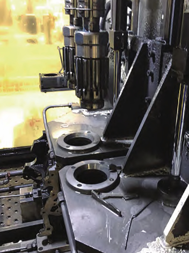
The defects in these images appear as bright fluorescent lines or clusters on a dark background. The challenging aspects include small crack width, non-uniform illumination, and background noise. The sample distribution is shown in the table below.
| Class | Training Images | Test Images |
|---|---|---|
| Defective | 1800 | 400 |
| Non-defective | 1000 | 200 |
| Total | 2800 | 600 |
3.2 Data Preparation and Database Creation
All images were resized to 227×227 pixels to match the network input. I created two directories under Caffe: train and val, each containing subdirectories for defective (y) and non-defective (w) samples. Label files (train.txt and val.txt) were generated with image paths and class labels. Then, the images were converted to LMDB database format using Caffe’s convert_imageset utility. A mean file was computed from the training set to normalize the data.
3.3 Initial Training and Hyperparameter Tuning
I first trained the baseline AlexNet model with default parameters. The solver configuration included:
- base_lr: 0.0018
- momentum: 0.9
- weight_decay: 0.0005
- test_iter: 80
- test_interval: 120
- max_iter: 12000
- stepsize: 4000
- gamma: 0.1
The initial accuracy reached 97.25%, which was promising but could be improved. I then systematically tuned the base learning rate and weight decay. The results are summarized in the table below.
| Exp | base_lr | weight_decay | Accuracy (%) |
|---|---|---|---|
| 1 | 0.01 | 0.0005 | 97.00 |
| 2 | 0.001 | 0.0005 | 97.00 |
| 3 | 0.003 | 0.0005 | 97.25 |
| 4 | 0.002 | 0.0005 | 98.00 |
| 5 | 0.0009 | 0.0005 | 97.75 |
| 6 | 0.0018 | 0.0005 | 98.25 |
The best learning rate was found to be 0.0018, giving an accuracy of 98.25%. Setting the learning rate too high causes the optimization to oscillate or diverge, while too low a rate leads to slow convergence and potentially suboptimal solutions.
3.4 Impact of Convolution Kernel Size
The size of the convolution kernel determines the receptive field of each neuron. For images with relatively large and distinct defect features, a larger kernel may capture more global context, whereas smaller defects require smaller kernels to preserve fine details. I conducted experiments by reducing and increasing the kernel sizes of the first three convolutional layers.
Experiment A: Decreased kernel sizes — conv1: 11→7, conv2: 5→5 (padding adjusted), conv3: 3→3. This resulted in an accuracy of 96.5%, which was worse than the baseline.
Experiment B: Increased kernel sizes — conv1: 11→13 (pad 0→1), conv2: 5→7 (pad 2→3), conv3: 3→5 (pad 1→2). This resulted in an accuracy of 98.75%, an improvement of 0.5% over the tuned baseline.
These results indicate that, for the magnetic particle images of sand foundry defects, larger kernels are beneficial, likely because the cracks span several pixels and require a broader neighborhood for reliable detection. The comparison is shown below.
| Experiment | Conv1 Kernel | Conv2 Kernel | Conv3 Kernel | Accuracy (%) |
|---|---|---|---|---|
| Baseline | 11 | 5 | 3 | 98.25 |
| Smaller kernels | 7 | 5 | 3 | 96.5 |
| Larger kernels | 13 | 7 | 5 | 98.75 |
3.5 Effect of Network Depth on Performance and Time Cost
Deeper networks can represent more complex functions but also require more computation and data. Since my classification task has only two classes, the depth of the standard AlexNet might be excessive. I hypothesized that removing some convolutional layers could reduce training time without sacrificing accuracy. In particular, conv3 and conv4 do not have corresponding pooling layers, and their removal simplifies the network. I removed both conv3 and conv4, resulting in a network with only 3 convolutional layers. The modified architecture is:
- Conv1 (13×13, pad 1, stride 4, output 96)
- Pool1 (3×3, stride 2)
- Conv2 (7×7, pad 3, stride 1, output 256)
- Pool2 (3×3, stride 2)
- Conv5 (5×5, pad 2, stride 1, output 256)
- Pool5 (3×3, stride 2)
- Fc6 (4096)
- Fc7 (4096)
- Fc8 (2)
The training time was reduced by approximately 29%, and the accuracy actually improved to 99%. The comparison is given in the table below.
| Model | Iterations | Accuracy (%) | Loss | Training Time (s) |
|---|---|---|---|---|
| Baseline (5 conv) | 12000 | 97.25 | 0.0961 | 1446 |
| Tuned baseline | 12000 | 98.25 | 0.0784 | 1385 |
| Larger kernels | 12000 | 98.75 | 0.0764 | 1367 |
| Removed conv3&4 | 12000 | 99.00 | 0.0780 | 966 |
This experiment demonstrates that a shallower architecture can outperform a deeper one when the task complexity is low. The simplified network is also more suitable for real-time embedded deployment due to its lower computational cost.
3.6 Pooling Method Comparison
I also compared max pooling and average pooling. In max pooling, the maximum value in each region is taken, which helps preserve strong features and reduces the influence of small pixel values. Average pooling averages all values, which can be more sensitive to noise. Replacing all max pooling layers with average pooling in my simplified network resulted in an accuracy of 98.25%, lower than the 99% achieved with max pooling. Therefore, max pooling was retained.
3.7 Analysis of Training Dynamics
For the best model (simplified network with larger kernels and max pooling), I plotted the accuracy and loss curves over time. The training loss and test loss decreased rapidly during the first 20 seconds, indicating fast learning. Between 20 and 600 seconds, the losses oscillated but generally decreased, showing continued convergence. After 600 seconds, both losses became stable at small values, indicating that the model had learned the underlying patterns. The relationship between training loss and test loss can be interpreted as follows:
| Train Loss | Test Loss | Network State |
|---|---|---|
| Decreasing | Decreasing | Still learning |
| Decreasing | Constant | Overfitting |
| Constant | Decreasing | Dataset issue |
| Increasing | Increasing | Network architecture has serious issues |
| Stable (small) | Stable (small) | Learning completed |
The final model achieved a training accuracy of 99% and a test accuracy of 98.75% on the validation set during training. The confusion matrix is shown below.
| Predicted Defective | Predicted Non-defective | |
|---|---|---|
| Actual Defective | 400 | 0 |
| Actual Non-defective | 8 | 192 |
This corresponds to a false-negative rate of 0%, which is critical for safety-critical components, and a false-positive rate of 4%.
4. Embedded System Implementation
4.1 Design Goals and Requirements
The goal of this phase was to build a compact and low-cost hardware system that could run the trained CNN model in real time. The functional requirements are:
- Acquire magnetic particle images and classify them as defective or non-defective.
- Output the classification result and display it on a screen.
- Achieve a missed detection rate of zero.
- Process each image within one second.
4.2 Hardware Components
The hardware system comprises the following components:
- Illumination: A LUYOR-3106 LED ultraviolet lamp provides uniform 365 nm UV light to excite the fluorescent magnetic particles.
- Camera: A Daheng MER-030-120UM industrial CCD camera with 656×492 resolution and 120 fps frame rate captures the images.
- Frame Grabber: A TC-542N1 PCIe frame grabber transfers image data to the embedded processor.
- Embedded Platform: NVIDIA Jetson TX1 development kit, which features a 256-core Maxwell GPU, 64-bit ARM A57 CPU, 4 GB LPDDR4 memory, and 16 GB flash storage.
- Display: An HDMI monitor for user interface and result display.
Jetson TX1 was chosen because its GPU provides 1 Teraflops of floating-point performance, sufficient for running the CNN inference in real time.
4.3 Software Environment Setup
I initialized the Jetson TX1 using NVIDIA JetPack, which installs Ubuntu for Tegra, CUDA, cuDNN, OpenCV, and other libraries. The steps included:
- Connecting the TX1 board to a host PC via a micro-USB cable and setting the board into forced recovery mode.
- Flashing the Linux for Tegra operating system through JetPack.
- Installing CUDA, OpenCL, and Caffe dependencies.
- Updating the apt sources to accelerate package downloads.
- Installing SSH server for remote login, and lrzsz for file transfer.
After the system was configured, I downloaded the Caffe source and compiled it with CUDA support. Then I copied the trained model files (including the network definition and weights) from the GTX 1080 workstation to the Jetson TX1.
4.4 Performance Testing on the Embedded System
I evaluated the embedded system using the test set of 600 images (400 defective, 200 non-defective). The results are summarized below.
| Defective | Non-defective | Total | |
|---|---|---|---|
| Test samples | 400 | 200 | 600 |
| Correctly classified | 400 | 192 | 592 |
| Misclassified | 0 | 8 | 8 |
| Accuracy (%) | 100 | 96 | 98.67 |
The overall accuracy was 98.67%, with a missed detection rate of 0%. The false-positive rate was 4% (8 non-defective images were classified as defective). These results satisfy the engineering requirements.
To further illustrate the inference process, I ran a sample test image through the system. The terminal output showed the probability of belonging to each class. For example, for a non-defective sample image, the model output “0.993 – w” and “0.007 – y”, meaning the algorithm correctly classified it as non-defective. The inference time per image was well below one second, meeting the real-time requirement.
5. Conclusion and Future Work
In this thesis, I presented a comprehensive study on the application of deep learning for sand foundry defects detection in precision castings. By leveraging GPU-accelerated CNN training, I optimized the network architecture and hyperparameters to achieve high detection accuracy. The key findings are:
- The use of a GPU significantly accelerates model training, enabling experimentation with large datasets.
- Hyperparameter tuning, especially the learning rate, can improve accuracy by about 1%.
- Larger convolution kernels are beneficial for detecting sand foundry defects because the cracks have relatively large spatial extents.
- Removing non-essential convolutional layers simplifies the network, reduces training time by about 29%, and even improves accuracy from 98.75% to 99%.
- Max pooling outperforms average pooling for this application.
The trained model was successfully ported to a Jetson TX1 embedded system, achieving a final test accuracy of 98.67% with zero missed defects. This demonstrates the practicality of deploying deep learning models for automated inspection of sand foundry defects in real production environments.
Future work could explore the following directions:
- Model visualization: Use feature map visualization and deconvolution to better understand what the network learns, potentially guiding further architecture improvements.
- Multi-class defect classification: Expand the system to distinguish between different types of sand foundry defects, such as cracks, blowholes, and shrinkage.
- Real-time tracking: Integrate the detection system with industrial robots or conveyor belts for fully automated inline inspection.
- Deployment optimization: Apply model compression techniques (e.g., pruning, quantization) to speed up inference and reduce power consumption.
In summary, this work demonstrates that deep learning can effectively address the challenges associated with manual magnetic particle inspection, providing a fast, accurate, and reliable solution for sand foundry defects detection in precision castings.