
In the field of materials science, the study of wear-resistant alloys, particularly white cast iron, has always been a focal point due to its extensive applications in industrial components subject to abrasive conditions. As a researcher deeply involved in fluid machinery and material design, I have long been intrigued by the complex interplay between chemical compositions and mechanical properties in white cast iron. Traditional approaches often rely on single-parameter analyses, such as examining the effect of individual elements like carbon or chromium on hardness or tensile strength. However, these methods fail to capture the synergistic relationships among multiple chemical elements, which can significantly influence the overall performance of white cast iron. This limitation prompted me to explore more holistic analytical frameworks, leading to the adoption of grey system theory—a powerful tool for handling uncertain systems with limited data. In this article, I present a novel perspective on analyzing the grey relationality among chemical compositions in wear-resisting white cast iron, introducing new concepts, methodologies, and computational techniques that can revolutionize how we optimize these materials. By leveraging grey relational analysis, I aim to uncover the intrinsic connections between elements like carbon (C), chromium (Cr), molybdenum (Mo), silicon (Si), manganese (Mn), vanadium (V), and copper (Cu), ultimately providing a theoretical foundation for enhancing material performance and facilitating product innovation.
White cast iron, renowned for its high hardness and excellent wear resistance, is widely used in manufacturing components such as pump parts, mill liners, and crushing equipment. The mechanical properties and microstructural characteristics of white cast iron are predominantly governed by its chemical composition and heat treatment parameters. Historically, research has focused on varying single elements or employing orthogonal experiments to assess their impact on properties like tensile strength and hardness. For instance, studies have shown that increasing carbon content can enhance hardness but may reduce toughness, while chromium addition improves corrosion and wear resistance. Yet, these investigations often overlook the interdependent relationships among chemical elements, which can lead to suboptimal material designs. In my previous work, I applied grey theory to analyze the comprehensive effects of chemical compositions on tensile strength and hardness in high-toughness ductile iron, revealing prioritized influencing factors. Building on that, I now extend this approach to wear-resisting white cast iron, proposing for the first time the concept of grey relationality among its chemical elements. This involves analyzing how elements correlate with each other, rather than just with performance metrics, using grey relational grades to quantify these associations. The methodology not only addresses the shortcomings of statistical methods that require large datasets and specific probability distributions but also offers a computationally efficient and robust alternative for material science research.
Grey system theory, established by Professor Deng Julong in 1982, is a transdisciplinary framework designed to study systems with partial information and uncertainty. Unlike probability theory or fuzzy logic, grey theory excels in scenarios with small samples and irregular data patterns, making it ideal for engineering applications where experimental data may be scarce. The core of grey relational analysis (GRA) is to measure the degree of correlation between factors in a system by comparing their behavioral sequences. In the context of white cast iron, the chemical elements can be treated as factors, with their concentration values forming data sequences. By calculating grey relational grades, we can determine which elements exhibit strong mutual influences, thereby guiding compositional adjustments for desired properties. The advantages of GRA are manifold: it does not require large sample sizes, avoids assumptions about data distribution, minimizes computational complexity, and ensures consistency between quantitative results and qualitative analysis. In this study, I employ a specific form of GRA called self-relational analysis, which constructs a matrix of relational grades among all element pairs without designating a reference sequence. This allows for a comprehensive exploration of the internal structure within the chemical composition of white cast iron.
To formalize the analysis, let me introduce the mathematical model underpinning grey relational analysis. Consider a system with m factors, each represented by a data sequence Xi = (xi(1), xi(2), …, xi(n)), where i = 1, 2, …, m, and n is the number of observations. For self-relational analysis, we compute the grey relational grade between every pair of sequences, resulting in a self-relational matrix s-r. This matrix is symmetric and has ones on its diagonal, reflecting self-correlation. The grey relational grade γ(Xi, Xj) between sequences Xi and Xj is calculated using the following steps, which I have adapted for white cast iron data.
First, normalize each sequence by converting it to its mean image or initial value image. This step eliminates scaling effects and ensures comparability. For a sequence Xi, the normalized sequence X’i is given by:
$$ X’_i = \left( \frac{x_i(1)}{\bar{x}_i}, \frac{x_i(2)}{\bar{x}_i}, \ldots, \frac{x_i(n)}{\bar{x}_i} \right) $$
where ̄xi is the mean of Xi. Alternatively, for simplicity, we can use the first value as a reference, but in this analysis, I employed the mean-based normalization to maintain consistency.
Second, compute the difference sequence between each pair of normalized sequences. The difference at point k is:
$$ \Delta_{ij}(k) = |x’_i(k) – x’_j(k)| $$
resulting in a difference sequence Δij = (Δij(1), Δij(2), …, Δij(n)).
Third, determine the environmental parameters: the maximum and minimum differences across all sequences and points. These are denoted as:
$$ M = \max_i \max_k \Delta_{ij}(k) $$
$$ m = \min_i \min_k \Delta_{ij}(k) $$
Fourth, calculate the grey relational coefficient for each point using the formula:
$$ \xi_{ij}(k) = \frac{m + \zeta M}{\Delta_{ij}(k) + \zeta M} $$
where ζ is the distinguishing coefficient, typically set to 0.5 to balance sensitivity and stability. This coefficient reflects the resolution between sequences; a higher ζ emphasizes differences, while a lower ζ smoothens them.
Fifth, obtain the grey relational grade by averaging the coefficients over all points:
$$ \gamma(X_i, X_j) = \frac{1}{n} \sum_{k=1}^n \xi_{ij}(k) $$
This grade ranges from 0 to 1, with values closer to 1 indicating stronger relationality. For self-relational analysis, we compute grades for all combinations of factors, leading to a matrix. If there are m factors, the number of combinations when taking two at a time is given by the binomial coefficient:
$$ C(m, 2) = \frac{m!}{2!(m-2)!} $$
which for m = 7 elements in white cast iron yields 21 unique pairs.
To apply this model to wear-resisting white cast iron, I gathered data from experimental studies on chemical compositions and tensile strength. The dataset includes seven chemical elements—C, Cr, Mo, Si, Mn, V, and Cu—along with tensile strength values, though the focus here is on the inter-element relationships. The data comprises seven groups, each representing a different composition variant, as summarized in the table below. This data serves as the foundation for calculating grey relational grades among the elements.
| Group | C (%) | Cr (%) | Mo (%) | Si (%) | Mn (%) | V (%) | Cu (%) | Tensile Strength (MPa) |
|---|---|---|---|---|---|---|---|---|
| 1 | 2.75 | 14.48 | 2.53 | 0.47 | 0.88 | 0.54 | 0.92 | 663 |
| 2 | 2.80 | 14.85 | 2.65 | 0.57 | 0.80 | 0.35 | — | 580 |
| 3 | 2.98 | 15.27 | 2.61 | 0.52 | 0.82 | 0.63 | 1.00 | 704.5 |
| 4 | 2.83 | 16.30 | 2.68 | 0.57 | 0.81 | 0.36 | — | 735 |
| 5 | 3.03 | 17.25 | 2.48 | 0.52 | 0.83 | 0.60 | 1.05 | 668.5 |
| 6 | 2.83 | 17.40 | 2.68 | 0.45 | 0.83 | 0.36 | — | 695.5 |
| 7 | 3.03 | 18.00 | 2.61 | 0.48 | 0.73 | 0.35 | — | 718.5 |
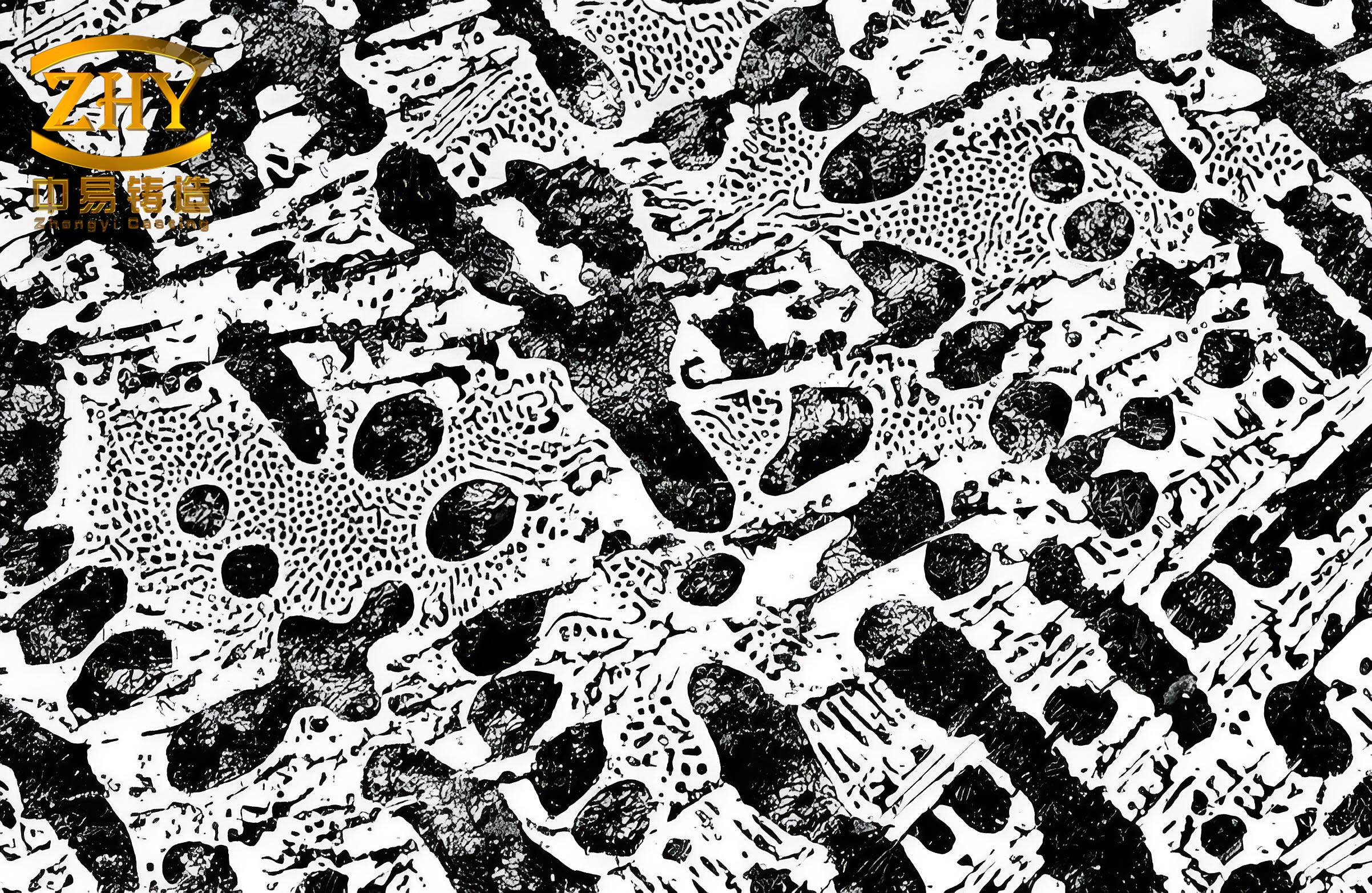
In this dataset, some entries for copper are missing, but for relational analysis among the seven elements, I handled the gaps by focusing on available data points and using normalization techniques to maintain consistency. The tensile strength is included for context, but the primary analysis centers on the chemical elements themselves. To visualize the microstructure of white cast iron, which often features carbides in a pearlitic or martensitic matrix, consider the following image that illustrates typical white cast iron morphology. This visual aids in understanding how chemical compositions influence microstructural development.
Proceeding with the calculation, I first normalized the data for each chemical element using the mean value method. This involved dividing each element’s values by its average across the seven groups to obtain dimensionless sequences. The normalized data, or initial value images, are presented in the table below. This step is crucial for eliminating units and scaling differences, allowing for fair comparison between elements.
| Group | C’ | Cr’ | Mo’ | Si’ | Mn’ | V’ | Cu’ |
|---|---|---|---|---|---|---|---|
| 1 | 1.0000 | 1.0000 | 1.0000 | 1.0000 | 1.0000 | 1.0000 | 1.0000 |
| 2 | 1.0182 | 1.0256 | 1.0474 | 1.2128 | 0.9091 | 0.6481 | — |
| 3 | 1.0836 | 1.0546 | 1.0316 | 1.1064 | 0.9318 | 1.1667 | 1.0870 |
| 4 | 1.0291 | 1.1257 | 1.0593 | 1.2128 | 0.9205 | 0.6667 | — |
| 5 | 1.1018 | 1.1913 | 0.9802 | 1.1064 | 0.9432 | 1.1111 | 1.1413 |
| 6 | 1.0291 | 1.2017 | 1.0593 | 0.9574 | 0.9432 | 0.6667 | — |
| 7 | 1.1018 | 1.2431 | 1.0316 | 1.0213 | 0.8295 | 0.6481 | — |
Next, I computed the difference sequences for all 21 element pairs. For example, for the pair C and Cr, the difference sequence ΔC-Cr is calculated by taking absolute differences between their normalized values across groups. This process was repeated for every combination, resulting in a set of difference sequences. From these, I derived the environmental parameters: the global maximum difference M = 0.595 and the global minimum difference m = 0, based on the data. With ζ = 0.5, the grey relational coefficients were then computed for each point using the formula:
$$ \xi_{ij}(k) = \frac{0 + 0.5 \times 0.595}{\Delta_{ij}(k) + 0.5 \times 0.595} = \frac{0.2975}{\Delta_{ij}(k) + 0.2975} $$
Finally, the grey relational grade for each pair was obtained by averaging the coefficients over the seven groups. The results are summarized in the self-relational matrix below, which encapsulates the relational grades between all element pairs. This matrix is symmetric, with diagonal entries equal to 1 (representing self-correlation), and off-diagonal entries indicating the degree of association.
| C | Cr | Mo | Si | Mn | V | Cu | |
|---|---|---|---|---|---|---|---|
| C | 1.0000 | 0.7953 | 0.8621 | 0.7887 | 0.7015 | 0.5593 | 0.9541 |
| Cr | 0.7953 | 1.0000 | 0.7549 | 0.7036 | 0.6041 | 0.8271 | 0.9155 |
| Mo | 0.8621 | 0.7549 | 1.0000 | 0.7671 | 0.6391 | 0.5317 | 0.8047 |
| Si | 0.7887 | 0.7036 | 0.7671 | 1.0000 | 0.6463 | 0.5310 | 0.9426 |
| Mn | 0.7015 | 0.6041 | 0.6391 | 0.6463 | 1.0000 | 0.6022 | 0.7163 |
| V | 0.5593 | 0.8271 | 0.5317 | 0.5310 | 0.6022 | 1.0000 | 0.8905 |
| Cu | 0.9541 | 0.9155 | 0.8047 | 0.9426 | 0.7163 | 0.8905 | 1.0000 |
From this matrix, we can extract the grey relational grades for each of the 21 element pairs. To facilitate interpretation, I have sorted these grades in descending order in the table below. This ranking reveals which element combinations exhibit the strongest or weakest relationalities in white cast iron, providing insights for material design.
| Rank | Grey Relational Grade | Element Pair | Interpretation |
|---|---|---|---|
| 1 | 0.9541 | C-Cu | Strongest association; carbon and copper are highly correlated. |
| 2 | 0.9426 | Si-Cu | Very strong relationality between silicon and copper. |
| 3 | 0.9155 | Cr-Cu | High correlation between chromium and copper. |
| 4 | 0.8905 | V-Cu | Strong relationality for vanadium and copper. |
| 5 | 0.8621 | C-Mo | Carbon and molybdenum show considerable association. |
| 6 | 0.8271 | Cr-V | Chromium and vanadium are moderately correlated. |
| 7 | 0.8047 | Mo-Cu | Molybdenum and copper have a notable relationship. |
| 8 | 0.7953 | C-Cr | Carbon and chromium exhibit moderate relationality. |
| 9 | 0.7887 | C-Si | Carbon and silicon are somewhat associated. |
| 10 | 0.7671 | Mo-Si | Molybdenum and silicon show a fair degree of correlation. |
| 11 | 0.7549 | Cr-Mo | Chromium and molybdenum have a relational grade in this range. |
| 12 | 0.7163 | Mn-Cu | Manganese and copper are moderately related. |
| 13 | 0.7036 | Cr-Si | Chromium and silicon exhibit a similar level of association. |
| 14 | 0.7015 | C-Mn | Carbon and manganese show a relational grade here. |
| 15 | 0.6463 | Si-Mn | Silicon and manganese have a weaker but notable correlation. |
| 16 | 0.6391 | Mo-Mn | Molybdenum and manganese are less strongly associated. |
| 17 | 0.6041 | Cr-Mn | Chromium and manganese exhibit a moderate relationality. |
| 18 | 0.6022 | Mn-V | Manganese and vanadium show a similar degree of correlation. |
| 19 | 0.5593 | C-V | Carbon and vanadium have a weaker association. |
| 20 | 0.5317 | Mo-V | Molybdenum and vanadium are minimally correlated. |
| 21 | 0.5310 | Si-V | Weakest relationality; silicon and vanadium show little correlation. |
The results highlight that the C-Cu pair has the highest grey relational grade (0.9541), indicating a strong synergistic relationship between carbon and copper in white cast iron. This suggests that variations in carbon content are closely tied to copper levels, possibly due to their combined effects on carbide formation and matrix hardening. Conversely, the Si-V pair has the lowest grade (0.5310), implying minimal interdependence; silicon and vanadium may act independently in influencing the microstructure of white cast iron. The other pairs fall between these extremes, with grades reflecting varying degrees of association. For instance, Cu-containing pairs generally show high grades, underscoring copper’s role in enhancing relationality with other elements. These findings have profound implications for optimizing white cast iron compositions. By focusing on element pairs with strong relationalities, such as C-Cu or Cr-Cu, material scientists can tailor compositions to achieve desired properties more efficiently. For example, adjusting copper levels might simultaneously influence carbon behavior, leading to improved wear resistance without compromising toughness.
To delve deeper, let’s consider the combinatorial aspects. For m = 7 elements, the number of unique pairs is calculated as:
$$ C(7, 2) = \frac{7 \times 6}{2} = 21 $$
which aligns with the 21 grades in the ranking. This combinatorial framework allows for systematic exploration of all possible interactions in white cast iron. In practice, when designing new alloys, engineers can use this grey relational analysis to prioritize element combinations that exhibit strong correlations, potentially reducing trial-and-error experiments. For instance, if the goal is to enhance hardness, one might focus on pairs like C-Cu or Cr-Cu, given their high relational grades, and adjust compositions accordingly. Moreover, this method can be extended to include more elements or additional performance metrics, such as impact toughness or corrosion resistance, by incorporating them into the grey relational model.
The application of grey theory to white cast iron analysis offers several advantages over conventional statistical methods. Traditional approaches like regression analysis or ANOVA require large datasets and assume normal distribution, which may not hold for small-sample material studies. In contrast, grey relational analysis thrives with limited data, making it ideal for preliminary investigations or when experimental resources are constrained. Additionally, the computational simplicity of GRA—involving basic arithmetic operations—enables quick insights without complex software. In my experience, this efficiency is invaluable for rapid material screening and optimization. Furthermore, the self-relational matrix provides a holistic view of internal dependencies, which is often missed in pairwise comparisons against a single reference. For white cast iron, this means we can understand not just how elements affect tensile strength, but how they interact with each other, leading to more coherent alloy design strategies.
Beyond white cast iron, the methodology presented here is applicable to a wide range of engineering materials and systems. For example, in other cast irons like ductile iron or steel alloys, grey relational analysis can elucidate chemical interactions and guide composition adjustments. It can also be used for process optimization, such as analyzing heat treatment parameters (e.g., temperature, time, cooling rate) and their effects on mechanical properties. The flexibility of grey theory allows it to adapt to various domains, from mechanical engineering to environmental science. In essence, by embracing this grey relational approach, researchers can uncover hidden patterns in complex systems, fostering innovation and efficiency in material development.
In conclusion, this study introduces a groundbreaking perspective on analyzing chemical compositions in wear-resisting white cast iron through grey relational analysis. By employing grey theory, I have quantified the relational grades among seven key chemical elements, revealing that carbon and copper share the strongest association, while silicon and vanadium exhibit the weakest. The self-relational matrix and ranked list provide a comprehensive map of inter-element relationships, offering valuable insights for optimizing white cast iron compositions. This novel approach addresses the limitations of traditional single-parameter analyses and opens new avenues for material science research. As we continue to explore the frontiers of alloy design, grey relational analysis will undoubtedly play a pivotal role in enhancing the performance and durability of white cast iron and other advanced materials. I encourage fellow researchers to adopt this methodology, leveraging its simplicity and power to drive innovation in their respective fields.