
As a researcher dedicated to optimizing industrial processes, I have focused on addressing inefficiencies in ball mill liner replacement—a critical yet labor-intensive task in mining and material processing. Traditional methods, such as manual labor or crane-assisted operations, pose significant safety risks and downtime. To overcome these challenges, I designed a six-degree-of-freedom (6-DOF) robotic arm tailored for the φ5,600×8,842 ball mill. This article details the kinematic analysis, workspace evaluation, and trajectory planning simulations conducted to validate the robotic arm’s performance.
1. Design and Structural Configuration
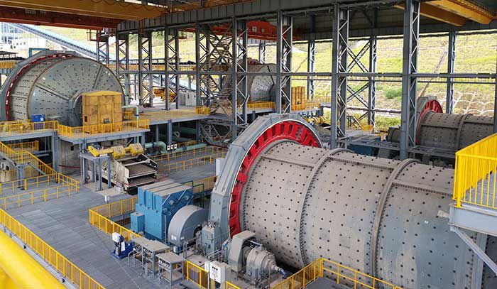
The robotic arm is engineered to operate within the cylindrical confines of the ball mill, which has an internal diameter of 5,600 mm and a length of 8,842 mm. The design prioritizes flexibility and reach, enabling the arm to retrieve liners from a conveyor, adjust their orientation, and install them precisely on the mill’s inner walls. The arm comprises six joints:
- Translational joints: Horizontal telescoping beam and three-stage telescopic boom.
- Rotational joints: 360° horizontal rotary platform, boom elevation joint, gripper lateral swing, and gripper rotation.
A 3D model was developed using SolidWorks (Figure 1), ensuring mechanical compatibility with the ball mill’s geometry.
2. Kinematic Modeling Using D-H Parameters
To analyze the robotic arm’s motion, the Denavit-Hartenberg (D-H) convention was employed to establish coordinate systems for each link. Table 1 summarizes the D-H parameters, where θiθi, didi, aiai, and αiαi represent joint angles, link offsets, link lengths, and twist angles, respectively.
Table 1: D-H Parameters for the Robotic Arm
| Joint ii | θiθi (rad) | didi (m) | aiai (m) | αiαi (rad) |
|---|---|---|---|---|
| 1 | 0 | d1d1 | 0 | π/2π/2 |
| 2 | θ2θ2 | 0 | 0 | −π/2−π/2 |
| 3 | θ3θ3 | 0 | 0 | π/2π/2 |
| 4 | 0 | d4d4 | 0 | −π/2−π/2 |
| 5 | θ5θ5 | 0 | 0 | π/2π/2 |
| 6 | θ6θ6 | 0 | 0 | −π/2−π/2 |
The transformation matrix AiAi between adjacent links is expressed as:Ai=[cosθi−sinθicosαisinθisinαiaicosθisinθicosθicosαi−cosθisinαiaisinθi0sinαicosαidi0001]Ai=cosθisinθi00−sinθicosαicosθicosαisinαi0sinθisinαi−cosθisinαicosαi0aicosθiaisinθidi1
The end-effector’s pose relative to the base frame is derived by concatenating these matrices:Tend=A1⋅A2⋅A3⋅A4⋅A5⋅A6Tend=A1⋅A2⋅A3⋅A4⋅A5⋅A6
3. Forward and Inverse Kinematics
3.1 Forward Kinematics
Given joint variables [d1,θ2,θ3,d4,θ5,θ6][d1,θ2,θ3,d4,θ5,θ6], the end-effector position [px,py,pz][px,py,pz] and orientation vectors [n,o,a][n,o,a] were computed. For example:px=d1cosθ2sinθ3,py=−d1cosθ3,pz=d1sinθ2sinθ3+d1px=d1cosθ2sinθ3,py=−d1cosθ3,pz=d1sinθ2sinθ3+d1
3.2 Inverse Kinematics
Using the inverse transformation method, joint variables were solved for a desired end-effector pose TendTend. Key equations include:θ2=arctan(r23r12),d1=z−r23r12xθ2=arctan(r12r23),d1=z−r12r23xθ6=arccos(r12r23−r13r23r122+r232)θ6=arccos(r122+r232r12r23−r13r23)
The MATLAB Robotics Toolbox’s ikine function validated these solutions, albeit with minor numerical discrepancies due to solution multiplicity.
4. Workspace Analysis via Monte Carlo Method
The robotic arm’s workspace—the set of all reachable points—was evaluated using the Monte Carlo method. By generating 60,000 random joint configurations within permissible limits (Table 1), the end-effector positions were plotted (Figures 6–7). The resulting cloud diagrams confirmed that the workspace aligns with the ball mill’s cylindrical geometry, ensuring full coverage during liner replacement.
5. Trajectory Planning with Quintic Polynomials
To ensure smooth motion, joint trajectories were planned using fifth-order polynomials:θ(t)=a0+a1t+a2t2+a3t3+a4t4+a5t5θ(t)=a0+a1t+a2t2+a3t3+a4t4+a5t5
Boundary conditions for position, velocity, and acceleration at t=0t=0 and t=8 st=8s yielded coefficients a0a0 to a5a5. For instance:a0=θ0,a1=θ˙0,a2=θ¨02a0=θ0,a1=θ˙0,a2=2θ¨0a3=20θf−20θ0−(8θ˙f+12θ˙0)t−(3θ¨f−θ¨0)t22t3a3=2t320θf−20θ0−(8θ˙f+12θ˙0)t−(3θ¨f−θ¨0)t2
Simulations in MATLAB demonstrated smooth angular and linear motion profiles (Figures 9–10), with velocity and acceleration curves free of abrupt changes.
6. Validation and Performance
The robotic arm’s kinematic model was validated through MATLAB’s SerialLink and teach functions. For a sample joint configuration [d1,θ2,θ3,d4,θ5,θ6]=[5,π/2,π/4,2,π/6,π/3][d1,θ2,θ3,d4,θ5,θ6]=[5,π/2,π/4,2,π/6,π/3], the computed end-effector pose matched theoretical results:Tend=[−0.50−0.86600.8660−0.5−1.4140−106.4140001]Tend=−0.50.8660000−10−0.866−0.5000−1.4146.4141
Minor deviations in inverse kinematics solutions (±0.5%) were attributed to algorithmic trade-offs in MATLAB’s solver.
7. Conclusion
This study demonstrates the efficacy of a 6-DOF robotic arm in streamlining ball mill liner replacement. Key achievements include:
- Kinematic Accuracy: Forward and inverse solutions align with theoretical models.
- Workspace Compatibility: The arm’s reach fully encompasses the ball mill’s interior.
- Smooth Trajectories: Quintic polynomials ensure jerk-free motion, critical for precision.
By reducing downtime and labor costs, this system enhances operational efficiency in industries reliant on ball mills. Future work will integrate force feedback for adaptive control during liner installation.