
1. Introduction
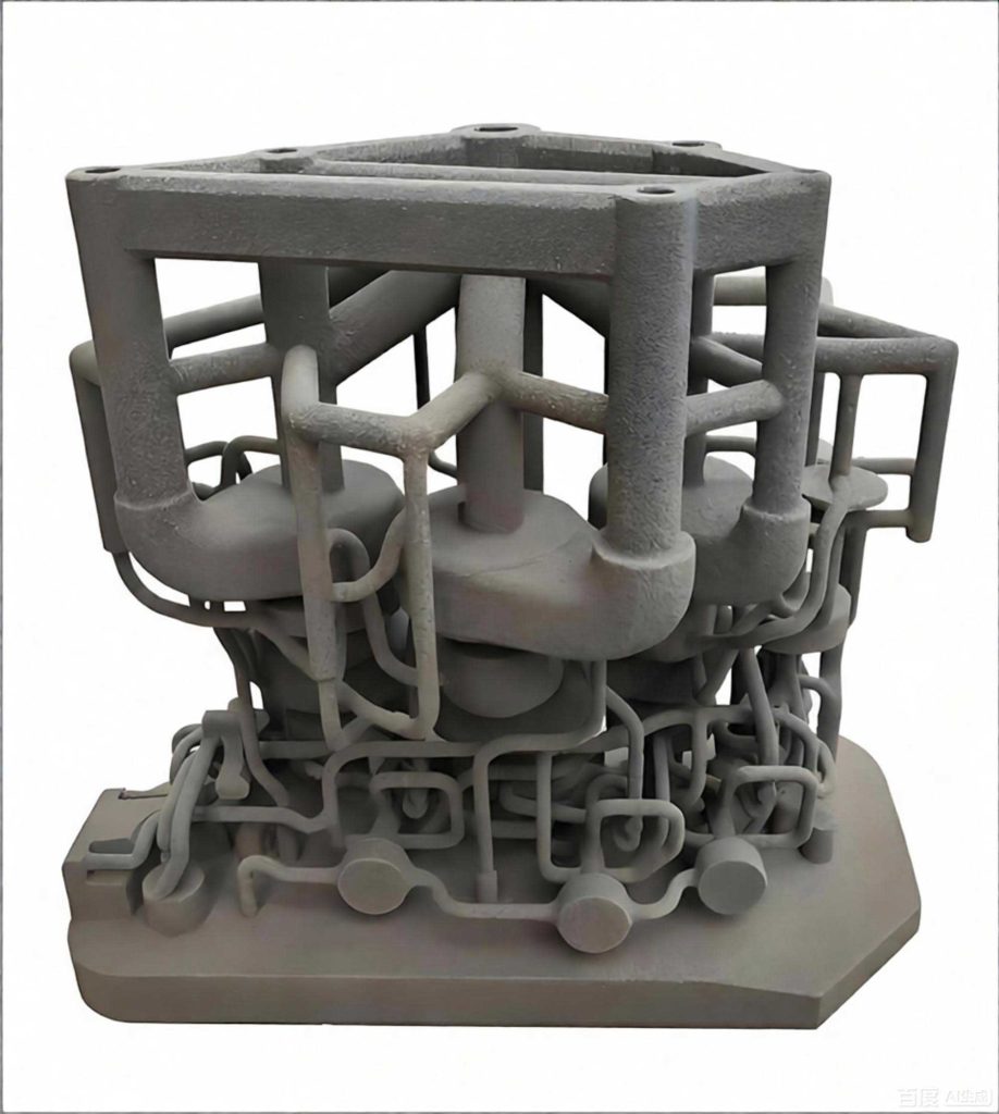
In the field of metal casting, sand mold 3D printing technology, also known as binder jetting additive manufacturing for sand molds, has emerged as a transformative approach that significantly improves the traditional sand casting workflow. Unlike conventional mold-making methods that rely on physical patterns and core boxes, 3d printing sand casting builds molds layer by layer directly from digital CAD data. This indirect forming technique offers numerous advantages, including high design freedom, reduced lead time, lower tooling costs, and the ability to produce complex internal geometries that would be difficult or impossible to achieve with traditional sand molding techniques.
The history of additive manufacturing dates back to the 1980s when early technologies such as stereolithography and selective laser sintering were developed. Among these, three-dimensional printing (3DP) technology, patented by Sachs et al. at the Massachusetts Institute of Technology in 1989, paved the way for binder jetting applications, including sand mold fabrication. In 3d printing sand casting, a print head selectively deposits a liquid binder onto a bed of sand particles that have been pre-mixed with a curing agent. The binder reacts with the curing agent to bond the sand grains, forming a solid mold layer by layer. After the printing process is complete, the unbound sand is removed and can be recycled, leaving a precisely shaped sand mold ready for metal pouring.
One of the most compelling aspects of 3d printing sand casting is its synergy with numerical simulation tools such as ProCAST. Because the mold geometry is created directly from CAD models, it is straightforward to perform finite element simulations of mold filling, solidification, and defect prediction before the actual casting is produced. This integration of simulation and additive manufacturing enables engineers to optimize the casting process in a virtual environment, reducing trial-and-error experiments and accelerating product development. Moreover, the technology is particularly advantageous for small-batch production and customized components, such as pump housings, impellers, valve bodies, and complex steel castings used in aerospace, marine, and energy industries.
Despite these benefits, several challenges remain in the practical application of 3d printing sand casting. The quality of the printed sand mold depends heavily on process parameters such as layer thickness, binder content, curing agent content, printing speed, and binder saturation. If these parameters are not properly optimized, the resulting mold may exhibit insufficient strength, excessive gas evolution, poor surface finish, or dimensional inaccuracies. Furthermore, the casting design—including gating system, riser placement, and chill positioning—must be carefully engineered to avoid defects such as shrinkage porosity, gas porosity, cold shuts, and misruns, especially for steel castings with thin walls and varying section thicknesses.
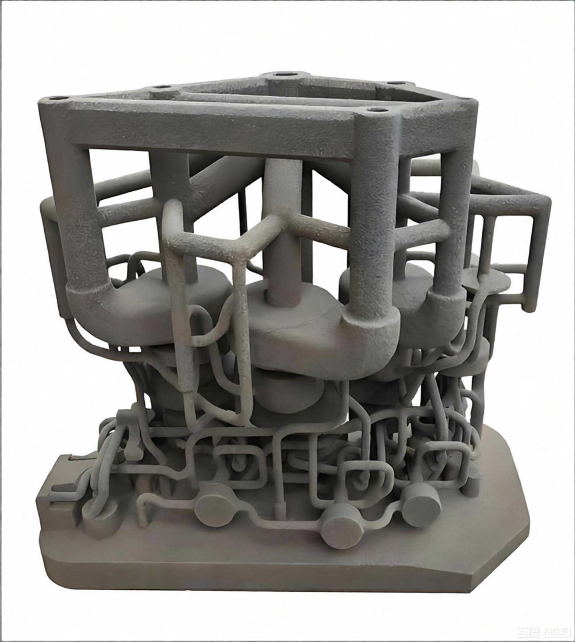
In this study, I focus on two key aspects of 3d printing sand casting: process parameter optimization and casting process design. First, I employ response surface methodology (RSM) to optimize the printing parameters of furan resin sand, specifically the layer thickness, furan resin content, and curing agent content, in order to achieve a sand mold with high tensile strength and low gas evolution. Second, I design the casting process for a natural gas meter housing made of 316 stainless steel, a thin-walled complex steel casting. Using ProCAST simulation software, I analyze three different gating system designs, evaluate filling and solidification behavior, predict shrinkage porosity, and finally improve the process by adding risers and chills. The results demonstrate that the combination of 3d printing sand casting with computational simulation can markedly enhance casting quality while minimizing defects.
2. Materials and Experimental Methods
2.1 Raw Materials
The sand used in this study was a special silica sand specifically formulated for 3D sand mold printing. Its properties are summarized in Table 1. The sand exhibited uniform particle size distribution, low acid demand, and low loss on ignition, which are beneficial for consistent binder curing and reduced gas generation during metal pouring.
| Property | Value |
|---|---|
| Moisture content (%) | 0.08 |
| Clay content (%) | 0.12 |
| Acid demand value (%) | 3.1 |
| Loss on ignition (%) | 0.15 |
| Bulk density (g/cm³) | 1.47 |
| SiO₂ content (%) | 99.6 |
| Fe₂O₃ content (%) | 0.023 |
| Al₂O₃ content (%) | 0.34 |
The binder system consisted of furan resin and a curing agent based on p-toluenesulfonic acid. Tables 2 and 3 list the main properties of the furan resin and curing agent, respectively.
| Property | Value |
|---|---|
| Moisture content (%) | 3.47 |
| Nitrogen content (%) | 0.02 |
| Density (g/cm³) | 1.151 |
| Viscosity at 20 °C (mPa·s) | 19 |
| Free formaldehyde (%) | 0.09 |
| Property | Value |
|---|---|
| Total acidity (%) | 0.08 |
| Density (g/cm³) | 0.12 |
| Free sulfuric acid (%) | 3.1 |
| Viscosity at 20 °C (mPa·s) | 0.15 |
2.2 Sand Mold 3D Printing Equipment
All sand specimens were printed using an HX1000 industrial sand mold 3D printer manufactured in China. The printer featured a build chamber of 1000 mm × 800 mm × 600 mm and employed a binder jetting process with a piezoelectric printhead array. The machine parameters could be adjusted within the following ranges: layer thickness from 0.25 mm to 0.4 mm, furan resin content from 0.5% to 2.0% by weight of sand, and curing agent content from 2‰ to 4‰ by weight of sand.
The printing procedure began with mixing the curing agent into the silica sand in a mixing chamber. The pre-mixed sand was then transferred to a storage hopper, from which a roller spread a uniform layer of sand onto the build platform. The printhead then selectively deposited the furan resin binder onto the sand bed according to the sliced CAD data. This cycle of spreading, printing, and lowering the build platform was repeated until the full mold was completed. After printing, the molds were allowed to cure naturally at room temperature for 24 hours before any testing was performed. Unbound sand was removed and recycled through a sieving system for subsequent reuse.
2.3 Testing Methods
The tensile strength of the printed sand specimens was measured using an XQY-II intelligent sand strength testing machine, which applied a continuously increasing mechanical load until specimen failure. The measurements were performed in accordance with the national standard GB/T 2684-2009 for foundry sands. The specimens were printed in a standard “8” shape with a gauge length of 50 mm and a cross-sectional area of 650 mm² at the neck, as specified by the standard. Eight specimens were tested for each condition, and the average tensile strength was recorded.
The gas evolution of the cured sand was measured using a GET-III intelligent gas evolution tester. Sand powder (1.00 g) was precisely weighed and placed in a porcelain boat, which was then inserted into the preheated furnace chamber at 850 °C. The gas pressure generated by the decomposition of organic components was measured by the change in system pressure. Six measurements were performed for each condition, and the average gas evolution value was reported.
2.4 Experimental Design
Because the quality of the 3D-printed sand mold depends on multiple interacting process parameters, I adopted response surface methodology to design the experiments and model the relationships between the input variables and the output responses. The three independent variables were: layer thickness (A), furan resin content (B), and curing agent content (C). The responses were tensile strength (Y₁) and gas evolution (Y₂).
I first conducted single-factor experiments to identify the reasonable range and center point for each variable. The center point was set at 0.35 mm layer thickness, 1.5% resin content, and 3.5‰ curing agent content. Subsequently, a three-factor, three-level Box-Behnken design was established with 17 experimental runs, including five replicates at the center point. The factors and their levels are summarized in Table 4.
| Factor | Level -1 | Level 0 | Level +1 |
|---|---|---|---|
| Layer thickness (mm) | 0.30 | 0.35 | 0.40 |
| Resin content (%) | 1.0 | 1.5 | 2.0 |
| Curing agent content (‰) | 3.0 | 3.5 | 4.0 |
The response surface model used in this study was a second-order polynomial model:
$$Y = \beta_0 + \sum_{i=1}^{n} \beta_i x_i + \sum_{i=1}^{n} \beta_{ii} x_i^2 + \sum_{i<j} +=""
3. Response Surface Optimization of 3D Printing Sand Casting Parameters
3.1 Single-Factor Experiments
In order to determine the center values for the response surface study, I performed single-factor experiments by varying one parameter at a time while keeping the other two parameters fixed.
3.1.1 Effect of layer thickness
For this experiment, the resin content was fixed at 2.0% and the curing agent content at 3.5‰. The layer thickness was varied from 0.30 mm to 0.40 mm in increments of 0.05 mm. As shown in Fig. 1, the tensile strength decreased continuously from 0.993 MPa to 0.626 MPa as the layer thickness increased. This decreasing trend can be attributed to a reduction in the number of layers and, consequently, a lower total amount of resin delivered into the sand bed. A thinner layer also produced a more compact sand structure and a more homogeneous distribution of the binder and curing agent, which strengthened the bonding bridges between sand grains.
Simultaneously, the gas evolution decreased from 12.9 mL/g to 10.8 mL/g with increasing layer thickness. Since furan resin decomposes at high temperature to generate volatile gases, the total gas amount is proportional to the resin content within the mold. A larger layer thickness resulted in a lower overall resin fraction and therefore less gas production. Based on the trade-off between mechanical strength and gas evolution, I selected 0.35 mm as the center point for the layer thickness.
3.1.2 Effect of furan resin content
With the layer thickness fixed at 0.35 mm and the curing agent at 3.5‰, the resin content was varied from 1.0% to 2.0%. The tensile strength increased almost linearly from 0.714 MPa to 1.011 MPa with increasing resin content. This is explained by the improved binder penetration and the formation of more bonding bridges between adjacent sand particles at higher resin fractions. The gas evolution also rose from 10.1 mL/g to 11.9 mL/g, because more organic resin was available to decompose during heating. A resin content of 1.5% was chosen as the center point, balancing the need for adequate strength and acceptable gas evolution.
3.1.3 Effect of curing agent content
The curing agent content was varied from 3.0‰ to 4.0‰ while the layer thickness and resin content were held at 0.35 mm and 1.5%, respectively. The tensile strength exhibited a gradual increase from 0.715 MPa at 3.5‰ to 0.731 MPa at 4‰, with a comparatively steep rise in the range of 3.0‰ to 3.5‰. This trend indicates that an insufficient amount of curing agent leads to incomplete cross-linking of the resin, whereas an excessive amount might accelerate the reaction too quickly and hinder resin penetration. The gas evolution increased substantially from 8.3 mL/g to 12.2 mL/g over the tested range, as excess curing agent introduced additional sulfur-containing gases and unreacted decomposition products. The center point was set at 3.5‰.
3.2 Response Surface Experimental Results
The Box-Behnken design produced 17 experimental runs, and the measured responses are listed in Table 5.
| Run | A: layer thickness | B: resin content | C: curing agent | Tensile strength (MPa) | Gas evolution (mL/g) |
|---|---|---|---|---|---|
| 1 | -1 | -1 | 0 | 0.682 | 10.8 |
| 2 | 1 | -1 | 0 | 0.535 | 9.4 |
| 3 | -1 | 1 | 0 | 1.071 | 13.6 |
| 4 | 1 | 1 | 0 | 0.518 | 12.3 |
| 5 | -1 | 0 | -1 | 0.712 | 8.8 |
| 6 | 1 | 0 | -1 | 0.533 | 7.8 |
| 7 | -1 | 0 | 1 | 1.011 | 14.2 |
| 8 | 1 | 0 | 1 | 0.468 | 11.9 |
| 9 | 0 | -1 | -1 | 0.426 | 8.6 |
| 10 | 0 | 1 | -1 | 0.586 | 8.1 |
| 11 | 0 | -1 | 1 | 0.679 | 11.8 |
| 12 | 0 | 0 | 0 | 0.754 | 9.9 |
| 13 | 0 | 0 | 0 | 0.714 | 11.9 |
| 14 | 0 | 0 | 0 | 0.634 | 12.7 |
| 15 | 0 | 0 | 0 | 0.628 | 11.9 |
| 16 | 0 | 0 | 0 | 0.681 | 12.4 |
| 17 | 0 | 0 | 0 | 0.637 | 11.5 |
3.3 Regression Model for Tensile Strength
Using the least squares method, the response function for tensile strength was fitted as:
$$Y_1 = -0.66 – 0.18A + 0.076B + 0.082C – 0.10AB – 0.091AC – 0.021BC + 0.056A^2 – 0.014B^2 – 0.034C^2$$
The results of the analysis of variance (ANOVA) for this model are shown in Table 6.
| Source | Sum of squares | df | Mean square | F value | P value | Significance |
|---|---|---|---|---|---|---|
| Model | 0.45 | 9 | 0.050 | 28.01 | 0.0001 | ** |
| A | 0.25 | 1 | 0.25 | 142.67 | <0.0001 | ** |
| B | 0.046 | 1 | 0.046 | 26.00 | 0.0014 | ** |
| C | 0.054 | 1 | 0.054 | 30.27 | 0.0009 | ** |
| AB | 0.041 | 1 | 0.041 | 23.26 | 0.0019 | ** |
| AC | 0.033 | 1 | 0.033 | 18.70 | 0.0035 | ** |
| BC | 1.81×10⁻⁴ | 1 | 1.81×10⁻⁴ | 1.02 | 0.3463 | – |
| A² | 0.016 | 1 | 0.013 | 7.49 | 0.0291 | * |
| B² | 7.82×10⁻⁴ | 1 | 1.81×10⁻⁴ | 1.12 | 0.5278 | – |
| C² | 4.90×10⁻⁴ | 1 | 4.90×10⁻³ | 2.77 | 0.1401 | – |
| Residual | 0.012 | 7 | 1.77×10⁻³ | 1.61 | 0.3212 | – |
| Lack of fit | 6.77×10⁻³ | 3 | 2.26×10⁻³ | |||
| Pure error | 5.62×10⁻³ | 4 | 1.41×10⁻⁴ | |||
| Total | 0.46 | 16 | ||||
| R² = 0.9730 | R²(adj) = 0.9382 | |||||
The model was highly significant with \(P<0.001\), while the lack of fit was insignificant (\(P=0.3212\)), indicating good agreement between the model predictions and the experimental data. The determination coefficient \(R^2=0.9730\) and the adjusted determination coefficient \(R^2_{adj}=0.9382\) were both close to unity, confirming the excellent fit of the regression model for predicting tensile strength.
From the ANOVA table, the order of significance of the factors affecting tensile strength was: layer thickness (A) > curing agent content (C) > resin content (B). Furthermore, the interaction terms AB (layer thickness × resin content) and AC (layer thickness × curing agent content) were significant, whereas the interaction BC (resin content × curing agent content) was not significant. This indicates that layer thickness plays the dominant role in determining the mechanical integrity of the printed sand mold in 3d printing sand casting.
3.4 Regression Model for Gas Evolution
The response function for gas evolution was fitted as:
$$Y_2 = 10.72 – 1.08A + 1.21B + 0.36C + 0.075AB + 0.025AC – 1.05BC – 0.54A^2 + 0.44B^2 – 0.61C^2$$
The ANOVA results for this model are listed in Table 7.
| Source | Sum of squares | df | Mean square | F value | P value | Significance |
|---|---|---|---|---|---|---|
| Model | 30.02 | 9 | 3.34 | 68.57 | <0.0001 | ** |
| A | 9.24 | 1 | 9.24 | 190.06 | <0.0001 | ** |
| B | 11.76 | 1 | 11.76 | 241.79 | <0.0001 | ** |
| C | 1.05 | 1 | 1.05 | 21.61 | 0.0023 | ** |
| AB | 0.023 | 1 | 0.023 | 0.46 | 0.5183 | – |
| AC | 2.50×10⁻³ | 1 | 2.50×10⁻³ | 0.051 | 0.8271 | – |
| BC | 4.41 | 1 | 4.41 | 90.66 | <0.0001 | ** |
| A² | 1.21 | 1 | 1.21 | 24.78 | 0.0016 | * |
| B² | 0.82 | 1 | 0.82 | 16.76 | 0.0046 | * |
| C² | 1.57 | 1 | 1.57 | 32.21 | 0.0008 | ** |
| Residual | 0.34 | 7 | 0.049 | 2.87 | 0.1673 | – |
| Lack of fit | 0.23 | 3 | 0.077 | |||
| Pure error | 0.11 | 4 | 0.027 | |||
| Total | 30.86 | 16 | ||||
| R² = 0.9888 | R²(adj) = 0.9744 | |||||
The gas evolution model was also highly significant, with an \(R^2\) value of 0.9888. The lack of fit was insignificant (\(P=0.1673\)), further confirming the adequacy of the model. All three linear terms (A, B, C) were highly significant, and the order of influence was: resin content (B) > layer thickness (A) > curing agent content (C). The interaction between resin content and curing agent content (BC) was the only significant interaction term for gas evolution.
3.5 Optimization and Verification
Using the established regression models, I performed a numerical optimization with the goal of maximizing tensile strength and minimizing gas evolution. The optimization routine suggested a layer thickness of 0.30 mm, a resin content of approximately 1.63%, and a curing agent content of 4‰, predicting a tensile strength of 1.071 MPa and a gas evolution of 11.04 mL/g.
Considering practical limitations of the printer and the desire for easy adjustability, I selected the following optimized parameters: layer thickness = 0.30 mm, resin content = 1.6%, and curing agent content = 4‰. Four verification experiments were conducted, and the results are shown in Table 8.
| Run | Layer thickness (mm) | Resin content (%) | Curing agent (‰) | Tensile strength (MPa) | Gas evolution (mL/g) |
|---|---|---|---|---|---|
| 1 | 0.3 | 1.6 | 4 | 1.063 | 11.0 |
| 2 | 0.3 | 1.6 | 4 | 1.049 | 11.3 |
| 3 | 0.3 | 1.6 | 4 | 1.050 | 11.2 |
| 4 | 0.3 | 1.6 | 4 | 1.058 | 10.9 |
| Average | 1.055 | 11.1 |
The measured average tensile strength and gas evolution were 1.055 MPa and 11.1 mL/g, respectively, which were in close agreement with the model predictions. This verification confirmed the reliability of the response surface models and the effectiveness of the optimization procedure for 3d printing sand casting.
4. Casting Process Design and Simulation for a Complex Steel Casting
4.1 Part Description and Casting Analysis
After optimizing the sand mold printing parameters, the next step was to design the casting process for a natural gas meter housing. The component was originally manufactured in ACD12 aluminum alloy, but was switched to 316 stainless steel (0Cr17Ni12Mo2) to improve corrosion resistance in demanding service conditions. The part has a cylindrical thin-wall geometry with a central partition plate, three side bosses, and one flanged boss. The wall thickness varies from 4 mm at the thin sections to 7 mm at the thicker sections, with a maximum thickness of 15 mm at the flange. The overall outer dimension is approximately 150 mm.
Because of the complex geometry and variable wall thickness, conventional sand molding would require multiple cores and precise core assembly, which is both costly and error-prone. 3d printing sand casting is particularly well suited for this component because the entire mold, including cores and internal channels, can be printed as an integrated structure. This eliminates cumulative assembly errors, improves dimensional accuracy, and reduces the manufacturing lead time.
4.2 Gating System Design
A closed-open gating system was adopted, featuring circular runner cross-sections to minimize heat loss during filling. Using the section-ratio design method, the cross-sectional area ratio of the sprue, runner, and ingate was determined as:
$$\frac{A_{\text{sprue}}}{A_{\text{runner}}} : \frac{A_{\text{runner}}}{A_{\text{ingate}}} : \frac{A_{\text{ingate}}}{A_{\text{ingate}}} = 11:9:10$$
The ingate area was calculated using the following formula:
$$A_{\text{ingate}} = \frac{G}{\mu \rho \tau \sqrt{2g H_p}}$$
where \(G\) is the total mass of molten metal flowing through the gating system, \(\rho\) is the density of the molten metal, \(\tau\) is the pouring time, \(\mu\) is the flow coefficient, and \(H_p\) is the average pressure head. For a middle injection system, the pressure head is given by:
$$H_p = H_0 – 0.5p$$
where \(H_0\) is the total height of the sprue and \(p\) is the height of the casting. The calculated sprue radius was 13 mm, subsequently adjusted to 15 mm for the sprue, 12 mm for the runner, and 13 mm for the ingate to improve filling efficiency and reduce the risk of gas entrapment.
Three gating system configurations were designed: (a) single-side injection, (b) bilateral injection, and (c) reverse bilateral injection. These three designs were intended to evaluate how the position and direction of the ingates influence filling uniformity and solidification behavior in this thin-walled steel casting.
4.3 Finite Element Simulation Setup
The three-dimensional solid models of the casting and gating systems were created in NX 12.0 and exported in Parasolid format. The geometry was then imported into ProCAST for mesh generation. Surface meshes were generated using triangular elements with a target edge length of 3 mm for the casting and 4 mm for the sand mold. Local mesh refinement was applied at the thin walls, at the sharp corners near the flanged boss, and in the vicinity of internal channels to ensure accurate geometric representation and heat transfer calculation.
The material properties of 0Cr17Ni12Mo2 steel were defined based on its chemical composition, shown in Table 9. Thermodynamic properties such as enthalpy, density, and solid fraction were calculated using the Lever rule within the ProCAST database.
| C | Si | Mn | P | S | Ni | Cr | Mo |
|---|---|---|---|---|---|---|---|
| ≤0.08 | ≤1.00 | ≤2.00 | ≤0.035 | ≤0.03 | 10.0-14.0 | 16.0-18.5 | 2.0-3.0 |
The mechanical properties of the steel are listed in Table 10. The liquidus temperature was 1505 °C, and the pouring temperature was set to 1560 °C to compensate for heat losses during filling. The sand mold was initially at room temperature (25 °C). The heat transfer coefficient between the casting and the sand mold was set to 1000 W m⁻² K⁻¹, while the coefficient between the casting and chills was set to 2000 W m⁻² K⁻¹. The exterior surfaces were treated as air-cooled boundaries.
| Property | Value |
|---|---|
| Tensile strength (MPa) | ≥520 |
| Yield strength (MPa) | ≥205 |
| Elongation (%) | ≥40 |
| Area reduction (%) | ≥60 |
| Density (g/cm³) | 7.98 |
| Specific heat at 20 °C (J g⁻¹ K⁻¹) | 0.502 |
The filling time was calculated based on the filling limit and flow conditions:
$$T = \frac{V \cdot \text{Fill Limit}(\%)}{100 \cdot s \cdot v}$$
where \(V\) is the cavity volume, \(s\) the cross-sectional area, and \(v\) the fluid velocity. The mass flow rate is related to the melt density and the total melt mass:
$$\dot{M} = V \cdot \frac{\text{Fill Limit}(\%)}{100} \cdot \rho(T)$$
$$\dot{M} = \frac{M}{T}$$
The total filling time was set to 4 s, with a total melt mass of 4.237 kg.
4.4 Governing Equations for Filling and Solidification
The filling flow of the molten metal was treated as an incompressible Newtonian fluid. The continuity equation is expressed as:
$$\frac{\partial u}{\partial x} + \frac{\partial v}{\partial y} + \frac{\partial w}{\partial z} = 0$$
where \(u\), \(v\), and \(w\) are the velocity components in the \(x\), \(y\), and \(z\) directions, respectively.
The momentum conservation is governed by the incompressible Navier–Stokes equation:
$$\rho \left( \frac{\partial \mathbf{v}}{\partial t} + (\mathbf{v} \cdot \nabla) \mathbf{v} \right) = \mathbf{F} – \nabla p + \mu \nabla^2 \mathbf{v}$$
where \(\mathbf{v}\) is the velocity vector, \(p\) is the pressure, \(\mu\) is the dynamic viscosity, and \(\mathbf{F}\) represents body forces.
The energy conservation equation during filling and solidification is:
$$\frac{\partial T}{\partial t} + u \frac{\partial T}{\partial x} + v \frac{\partial T}{\partial y} + w \frac{\partial T}{\partial z} = \frac{\lambda}{\rho c_p} \left( \frac{\partial^2 T}{\partial x^2} + \frac{\partial^2 T}{\partial y^2} + \frac{\partial^2 T}{\partial z^2} \right) + \frac{Q}{\rho c_p}$$
where \(T\) is the temperature, \(\lambda\) is the thermal conductivity, \(c_p\) is the specific heat, and \(Q\) is the latent heat source term:
$$Q = \rho L \frac{\partial f_s}{\partial T}$$
with \(L\) being the latent heat of fusion and \(f_s\) the solid fraction.
In the numerical implementation, the heat conduction equation is discretized using the finite element method:
$$M \frac{dT}{dt} + K T = F$$
where \(M\) is the mass matrix, \(K\) is the stiffness matrix, \(F\) is the external load vector, and \(T\) is the nodal temperature vector.
To predict shrinkage porosity in the casting, the Niyama criterion was employed:
$$M = \frac{G}{\sqrt{R}}$$
where \(G\) is the temperature gradient and \(R\) is the cooling rate. When the local value of \(M\) falls below a critical threshold (typically \(M \le 1.0\)), the risk of shrinkage porosity is considered high. ProCAST uses this criterion to map regions of potential micro-porosity.
4.5 Results of the Casting Simulation
4.5.1 Filling behavior
The flow field simulations of the three gating system designs are summarized below.
For the single-side injection scheme (Scheme A), at 1 s of filling, the melt entered the mold and concentrated on the right side of the cavity. The flow velocity near the inner wall was relatively high, but the flow near the bosses and thin-walled sections was slow, below 0.5 m/s. The filling was visibly asymmetric. At 2 s, the melt had covered about two-thirds of the cavity, but an obvious flow front stagnation was observed in the middle section, which increased the risk of cold shuts. By 3 s, the lower portion of the casting was fully filled, but the melt surface on the right was higher than on the left. At 4 s, the cavity was completely filled, but the overall filling sequence was disorderly.
For the bilateral injection scheme (Scheme B), at 1 s, the melt was still traveling through the runner. At 2 s, the melt entered the cavity from both sides simultaneously, and the liquid levels on both sides rose uniformly. The flow velocity in the lower thin-wall region was about 0.5 m/s and gradually stabilized. At 3 s, the melt had filled the main cavity evenly, with no significant height difference between the two sides. At 4 s, the filling was completed smoothly, with a relatively uniform velocity field and minimal turbulence. The bilateral arrangement reduced the filling distance and provided a balanced flow pattern.
For the reverse bilateral injection scheme (Scheme C), the melt entered the cavity at 1 s and immediately flowed toward the flange side. By 2 s, the flanged region was filled, but the high velocity difference across the cross-section (0.2 to 0.6 m/s) generated local turbulence near the boss, which could lead to gas entrapment and oxide inclusions. The filling at 3 s was still in progress, as several thin-walled areas remained unfilled. At 4 s, the casting was not yet completely filled, especially in the upper thick sections, indicating insufficient feeding capacity.
Overall, Scheme B demonstrated the most balanced filling behavior, with consistent velocity distribution and simultaneous advancement of the melt front on both sides, making it the preferred configuration for this component.
4.5.2 Solidification and temperature field analysis
Scheme A showed a non-uniform solidification pattern. The outer wall solidified progressively from the outside inward, but the central partition plate and the flanged boss solidified earlier than the surrounding areas. A thick isolated liquid region formed near the lower thin plate and remained molten long after the surrounding metal had solidified. The temperature field at 115 s showed that the lower section of the casting was still at about 1384 °C, while the surrounding regions had cooled below the liquidus temperature. This isolated pool of liquid metal inevitably led to shrinkage cavities and misruns.
Scheme B resulted in a much more uniform solidification sequence. The casting solidified from the thin center outward, following a progressive or directional solidification pattern. The flange area, with the largest thermal mass, solidified last at approximately 71 s, while the thin central sections solidified in about 9 s. The temperature field at 57 s and 147 s showed consistent temperature gradients across the casting, with no isolated liquid regions. The overall solidification time span was relatively narrow, which promoted uniform microstructure and reduced the probability of shrinkage defects.
Scheme C exhibited poor solidification uniformity. The solidification time varied significantly across the component, with some thin-walled areas taking over 100 s to solidify. The lower boss region formed a large isolated liquid pool as a result of insufficient melt feeding. By 143 s, some areas were still above 1260 °C, while the rest of the casting had already solidified. This large solidification gradient is unfavorable for soundness and dimensional accuracy.
4.5.3 Shrinkage porosity prediction
The defect predictions for the three schemes are summarized in Table 11.
| Parameter | Scheme A | Scheme B | Scheme C |
|---|---|---|---|
| Total defect volume (cc) | 3.533 | 3.445 | 2.476 |
| Shrinkage porosity volume (cc) | 0.559 | 0.391 | 0.499 |
| Density of defect (g·cc⁻¹, air) | 1.20 | 1.20 | 1.20 |
| Weight of defect (mg) | 0.671 | 0.469 | 0.599 |
Scheme A had the largest shrinkage porosity, reaching 0.559 cc, with defects distributed in the lower thick plate and around the flanged boss. Scheme B showed a lower shrinkage porosity volume of 0.391 cc, concentrated mainly in the flange area, which is accessible for riser feeding. Scheme C produced a defect volume of 0.499 cc, with scattered porosities in the work surfaces and some micro-porosity at the center of the casting.
Based on these results, Scheme B was selected as the most promising gating system for further optimization, since it offered the lowest defect volume and the most concentrated defect locations, thereby requiring the least amount of feed metal and the simplest modification.
5. Casting Process Improvement
5.1 Riser Design
To eliminate the concentrated shrinkage defects in the flanged boss region, I designed two open-top cylindrical risers placed on the top surface of the flange. The riser dimensions were determined using the modulus method:
$$M_{\text{riser}} = \frac{V_{\text{riser}}}{A_{\text{riser}}}$$
where \(V_{\text{riser}}\) is the volume and \(A_{\text{riser}}\) is the surface area of the riser. The calculated riser modulus was 3.8 mm. Using the thermal circle method, the riser diameter was calculated as 29 mm, and the height was set to 35 mm according to the empirical relationship \(H = 1.15 \sim 1.8D\). Fillets with a radius of 4 mm were applied at both top and bottom edges of the riser to reduce stress concentrations and facilitate melt flow. The riser geometry is shown in Fig. 4.
Table 12 lists the final riser parameters.
| Parameter | Symbol | Value |
|---|---|---|
| Riser modulus | M | 3.8 mm |
| Riser diameter | D | 29 mm |
| Riser height | H | 35 mm |
| Fillet radius (top) | r₁ | 4 mm |
| Fillet radius (bottom) | r₂ | 4 mm |
5.2 Chill Design
In addition to the risers, a steel chill was placed in the thick lower section of the casting to accelerate local solidification and prevent the formation of isolated liquid pools. The chill dimensions were determined based on the geometry of the thick section. The chill was 40 mm long, 20 mm wide, and 10 mm thick, as shown in the schematic drawing. The chill was positioned in direct contact with the casting surface, and the interface heat transfer coefficient was set to 2000 W·m⁻²·K⁻¹.
5.3 Casting Tolerances and Machining Allowance
According to the casting process design handbook, the following parameters were determined for this 316 stainless steel casting: the dimensional tolerance grade was CT13, corresponding to a tolerance value of 10 mm; the weight tolerance grade was M13, corresponding to a weight tolerance value of 24%; the machining allowance grade was 13/J, giving a machining allowance of 9 mm based on the basic dimension of 150 mm; and the process correction allowance for the flange region was 2 mm.
| Parameter | Value/grade |
|---|---|
| Dimensional tolerance grade | CT13 |
| Dimensional tolerance value | 10 mm |
| Weight tolerance grade | M13 |
| Weight tolerance value | 24% |
| Machining allowance grade | 13/J |
| Machining allowance | 9 mm |
| Process correction allowance (flange) | 2 mm |
6. Simulation of the Improved Casting Process
After adding the risers and chills to the selected bilateral injection gating system (Scheme B), the improved casting process was re-simulated in ProCAST with the same boundary conditions and material definitions. Table 14 lists the assigned material types and initial temperatures.
| Name | Type | Material | Initial temperature |
|---|---|---|---|
| Part (casting) | Alloy | 316 stainless steel | 1560 °C |
| Sand mold | Mold | Furan resin sand | 25 °C |
| Chill | Mold | Iron | 25 °C |
6.1 Filling Behavior of the Improved Casting
The improved filling simulation is shown in Fig. 5. Compared with the original unoptimized Scheme B, the optimized casting demonstrated more uniform melt velocity after entering the cavity. The problem of abnormally slow solidification at the lower thick wall was resolved. The melt velocity stabilized in the range of 0.5-0.8 m/s, and no significant height difference was observed between the two sides of the melt front. By 3 s, nearly the entire cavity had been filled, and the remaining volume was filled smoothly by 4 s. The risers promoted a continuous supply of molten metal to the flange region, thereby reducing the risk of premature solidification and shrinkage.
6.2 Solidification and Temperature Field of the Improved Casting
The improved solidification simulation is shown in Fig. 6. During the early stage of solidification, the lower thick section, in contact with the chill, solidified first as intended. This followed the principle of directional solidification, in which the lower portions solidify before the upper portions, and the risers remain liquid until the end to provide feeding. The temperature field showed that at 17 s, the lower portion had already cooled below the liquidus temperature. By 67 s, the solidification front had moved uniformly upward from the bottom and from the thin walls toward the thicker sections. At 147 s, the entire casting had solidified, with no isolated liquid regions remaining. The solidification process followed a clear bottom-to-top sequence, which is favorable for reducing shrinkage porosity.
6.3 Shrinkage Porosity of the Improved Casting
The predicted shrinkage porosity of the optimized casting is shown in Fig. 7. The defect distribution was drastically reduced. The shrinkage porosity inside the casting was only 0.0008 cc, while the defects that did occur were concentrated in the risers, with a volume of 0.073 cc. The comparison between the original and optimized processes is presented in Table 15.
| Parameter | Before optimization | After optimization |
|---|---|---|
| Shrinkage porosity in casting (cc) | 0.391 | 0.0008 |
| Shrinkage porosity in riser (cc) | – | 0.073 |
| Total shrinkage porosity (cc) | 0.391 | 0.0738 |
The overall defect content was reduced by more than 80%, and the residual porosity in the casting itself was negligible. This confirms that the designed riser and chill system, combined with the bilateral gating system, is highly effective in eliminating casting defects in this thin-walled stainless steel component fabricated via 3d printing sand casting.
7. Conclusion
In this research, I systematically investigated the process optimization of 3d printing sand casting, combining response surface methodology with finite element simulation to improve both the sand mold quality and the final casting soundness. The main conclusions are as follows:
1. The response surface methodology was successfully applied to optimize the printing parameters of furan resin sand for sand mold 3D printing. The optimal parameter set was determined as: layer thickness of 0.30 mm, furan resin content of 1.6% by weight of sand, and curing agent content of 4‰ by weight of sand. Under these conditions, the tensile strength of the printed sand mold reached 1.055 MPa, and the gas evolution was 11.1 mL/g, which agreed well with the model predictions.
2. The regression models revealed that layer thickness had the greatest influence on tensile strength, followed by curing agent content and resin content. In contrast, resin content was the dominant factor affecting gas evolution. Significant interaction effects were found between layer thickness and resin content for strength, and between resin content and curing agent content for gas evolution. These findings provide quantitative guidance for parameter selection in practical 3d printing sand casting production.
3. The casting process design for a natural gas meter housing was carried out using ProCAST simulation. A closed-open gating system with a circular cross-section was designed, and three filling configurations were evaluated: single-side injection, bilateral injection, and reverse bilateral injection. The bilateral injection scheme exhibited the most uniform filling, the steadiest solidification temperature gradient, and the lowest defect volume among the three designs, with shrinkage porosity of 0.391 cc.
4. Defect-oriented process improvement was performed by adding two open-top risers above the flanged boss and a steel chill at the thick lower section. The riser diameter was 29 mm and the height 35 mm. Casting process parameters such as dimensional tolerance, weight tolerance, machining allowance, and process correction allowance were determined based on standardized guidelines.
5. After optimization, the simulation results showed that the filling process became more uniform, the solidification time was significantly shortened, and the directional solidification pattern was clearly established. The shrinkage porosity inside the casting decreased from 0.391 cc to 0.0008 cc, while the remaining porosity was confined to the risers at 0.073 cc. This dramatic improvement demonstrates the effectiveness of combining 3d printing sand casting with numerical simulation, providing a robust reference for producing complex thin-walled steel castings with high quality and reliability.