
As a fundamental manufacturing process, sand casting remains one of the most versatile and widely adopted methods for producing metal components. Yet, the quality of sand castings is frequently jeopardized by shrinkage defects, which originate during the solidification stage when liquid metal contraction and solidification contraction cannot be fully compensated by liquid feeding. The accurate prediction of such defects is crucial for minimizing scrap and optimizing casting design. In this work, I focus on the sandy foundry defect problem, particularly shrinkage cavities and porosity, and present several algorithmic improvements to numerical simulation models. My goal is to improve both computational accuracy and efficiency for the prediction of sand foundry defect phenomena. The proposed models include a macro shrinkage degree algorithm, a macro-micro coupled porosity degree algorithm, and a dynamic grid technology model. Throughout this article, the term “sand foundry defect” will appear repeatedly to emphasize the practical context and the relevance of the simulations to real foundry production.
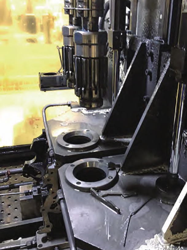
Figure 1 below illustrates a typical sand-cast engine cylinder block, where shrinkage defects are often concentrated in hot spots and poorly fed regions. This example serves as a reminder of the industrial importance of reliable defect prediction.
1. Introduction
Sand foundry defect control is a central issue in the casting industry. Shrinkage cavities and porosity are among the most severe internal discontinuities that degrade mechanical properties and pressure tightness. Numerical simulation has become an indispensable tool to visualize the solidification process and to predict where such defects might appear. However, traditional simulation methods often suffer from a trade-off between computational speed and accuracy. When a casting is large or geometrically complex, fine meshes are necessary to resolve defect morphologies, but the corresponding increase in mesh count and reduction in time step can make the simulation extremely slow. To address this problem, I have developed several enhanced algorithms within a self-developed casting simulation framework, which is originally designed for sand foundry defect prediction. This framework, written in Visual C++ and integrated with OpenGL for visualization, provides a flexible platform for testing new computational ideas.
2. Research Approach and Algorithm Foundation
My research follows two parallel directions: improving defect prediction accuracy and increasing computational efficiency. For the former, I propose a macro shrinkage degree concept that allows shrinkages to be distributed continuously over the top liquid pools, thereby avoiding an all-or-nothing grid-blocking approach. For the latter, I propose a dynamic grid technology that uses coarse grids for the thermal field calculation and locally refined grids for defect identification. In addition, I couple the macroscopic temperature field with a microscopic cellular automaton model to obtain a more physically realistic porosity evolution. All these efforts aim at a better characterization of sand foundry defect in terms of position, shape, and volume fraction.
The governing equation for the solidification process is the three-dimensional transient heat conduction equation with latent heat source:
$$ \rho c_p \frac{\partial T}{\partial t} = \lambda \left( \frac{\partial^2 T}{\partial x^2} + \frac{\partial^2 T}{\partial y^2} + \frac{\partial^2 T}{\partial z^2} \right) + Q $$
where \(T\) is temperature, \(t\) is time, \(\lambda\) is thermal conductivity, \(\rho\) is density, \(c_p\) is specific heat, and \(Q\) is the volumetric heat source due to solidification. The finite difference method is employed to discretize the equation. For a uniform mesh with spatial step \(\Delta x = \Delta y = \Delta z = \Delta l\), the explicit difference scheme in three dimensions can be written as:
$$ T_{i,j,k}^{n+1} = T_{i,j,k}^{n} + \frac{\lambda \Delta t}{\rho c_p (\Delta l)^2} \left[ \sum_{neighbors} \left( T_{neighbor}^{n} – T_{i,j,k}^{n} \right) \right] + \frac{Q \Delta t}{\rho c_p} $$
To ensure stability, the time step must satisfy the following condition:
$$ \frac{\lambda \Delta t}{\rho c_p (\Delta l)^2} \le \frac{1}{6} $$
This stability criterion implies that doubling the spatial resolution requires a time step reduction by a factor of four and an eightfold increase in mesh count, leading to a computational cost increase of roughly 30 to 50 times. This is the core motivation for my dynamic grid model.
The latent heat release during solidification is treated using a modified temperature recovery method. For hypoeutectic aluminum-silicon alloys, I separate the primary phase and eutectic phase contributions. The solid fraction is tracked using the Scheil-Gulliver model for the primary phase:
$$ f_{sP} = 1 – \left( \frac{T_m – T}{T_l – T} \right)^{\frac{1}{k_0 – 1}} $$
where \(T_m\) is the melting point of the solvent, \(T_l\) is the liquidus temperature of the alloy, and \(k_0\) is the equilibrium partition coefficient. The eutectic solid fraction evolution is computed with a continuous nucleation model and an Avrami-type growth law. The released latent heat is then converted into a temperature rise:
$$ \Delta T_{recovery} = \frac{L_P \rho_P \Delta f_{sP} + L_E \rho_E \Delta f_{sE}}{\rho c_p} $$
where \(L_P\) and \(L_E\) are the latent heats of the primary and eutectic phases, and \(\Delta f_{sP}\) and \(\Delta f_{sE}\) are the increments of the corresponding solid fractions.
3. Macro Shrinkage Degree Model
In conventional shrinkage cavity prediction, the algorithm compares the total shrinkage volume of each molten pool with the volume of the topmost liquid cell. If the shrinkage volume exceeds the cell volume, that cell is directly marked as a shrinkage cavity. This method has two drawbacks. First, cells that have already solidified are considered fully solid even if they contain a partially distributed shrinkage. Second, the predicted cavity shape strongly depends on the mesh orientation and size, often producing jagged boundaries. To overcome these issues, I introduce the concept of “shrinkage degree” for each grid cell. The shrinkage degree represents the volume fraction of shrinkage that has accumulated in a cell relative to the total cell volume. The algorithm proceeds as follows.
During each time step, the total shrinkage volume of a molten pool is calculated as:
$$ \Delta V = \Delta V_l + \Delta V_s $$
where the liquid contraction \(\Delta V_l\) and solidification contraction \(\Delta V_s\) are given by:
$$ \Delta V_l = \alpha V (1 – f_s) \Delta T $$
$$ \Delta V_s = \beta V \Delta f_s $$
Here, \(\alpha\) is the liquid volumetric contraction coefficient, \(\beta\) is the solidification contraction coefficient, \(V\) is the nominal volume of the cell, \(f_s\) is the solid fraction, and \(\Delta T\) and \(\Delta f_s\) are the changes in temperature and solid fraction during the time step.
Instead of assigning the entire shrinkage to the top cell only when it completely fills, I distribute the shrinkage volume equally among all currently active top pool cells. Each cell receives an increment of shrinkage degree:
$$ \Delta d_{sh} = \frac{\Delta V}{n_{top}} $$
where \(n_{top}\) is the number of cells in the top layer of the molten pool. The shrinkage degree \(d_{sh}\) of each cell is accumulated over time. When \(d_{sh}\) reaches 1.0, the cell is marked as a fully developed shrinkage cavity, and the remaining shrinkage volume is carried over to the next iteration. This real-time consumption approach allows cells that were previously judged as “fully filled” to retain a fractional shrinkage volume, which is more physically realistic.
Table 1 summarizes the key differences between the original shrinkage prediction method and the proposed macro shrinkage degree method.
| Aspect | Original Method | Macro Shrinkage Degree Method |
|---|---|---|
| Shrinkage distribution | Accumulated and applied to top cell when threshold reached | Uniformly distributed over top pool cells every time step |
| Grid dependency | High, cavity shape follows mesh edges | Low, cavity contour can be interpolated from shrinkage degree field |
| Handling of solidified cells | Treated as completely solid | May retain a fractional shrinkage degree |
| Accuracy | Limited by mesh size | Improved, closer to experimental cross-sections |
To validate the model, I conducted a wedge-shaped casting experiment using ductile iron. The mold material was graphite, and the pouring temperature was 1360°C. The simulation parameters are presented in Table 2.
| Parameter | Value |
|---|---|
| Spatial step | 2 mm |
| Number of grids | 1,755,000 |
| Pouring temperature | 1360 °C |
| Mold initial temperature | 200 °C |
| Environment temperature | 20 °C |
| Pouring time | 5 s |
| Casting material | QT450 |
| Mold material | Graphite |
After solidification, the casting was sectioned along its central plane. The comparison between the simulated shrinkage degree field and the actual casting cross-section showed that the new method yields a cavity depth and shape that are much closer to the experimental results. The traditional method predicted a deeper and more irregular cavity, while the shrinkage degree field provided a smoother contour that resembles the actual defect morphology. Thus, the macro shrinkage degree model effectively improves the prediction accuracy of sand foundry defect for ductile iron castings.
4. Macro-Micro Coupled Porosity Degree Model
Porosity (also called micro-shrinkage) is another form of sand foundry defect that appears as fine dispersed voids between dendrites. The formation of porosity is closely related to the dendritic network and the feeding resistance in the mushy zone. Macroscopic criteria such as the Niyama criterion can predict the location of porosity, but they cannot provide the porosity fraction or the microstructural morphology. To overcome this limitation, I developed a coupled macro-micro model that combines the macroscopic heat-transfer simulation with a cellular automaton (CA) model for microstructure evolution. The spatial and temporal synchronization between the two scales is achieved by introducing an operation order \(N_s\), defined as the number of microscopic time steps per macroscopic step:
$$ N_s = \frac{\Delta t_{macro}}{\Delta t_{micro}} $$
In my implementation, the macroscopic time step is \(\Delta t_{macro} = 0.003\) s and the microscopic time step is \(\Delta t_{micro} = 0.001\) s, so \(N_s = 3\). The cooling rate for the microscale model is extracted from the macroscopic temperature field:
$$ \dot{T} = \frac{\Delta T_{macro}}{N_s \Delta t_{micro}} $$
where \(\Delta T_{macro}\) is the temperature change during one macroscopic step. This ensures that the dendritic growth in the CA simulation follows a real cooling curve with true thermal history, instead of using a constant cooling rate assumption.
For the porosity prediction, I employ a criterion based on local pressure loss. According to Darcy’s law, the pressure drop for liquid flow through the dendritic network is:
$$ \Delta P = \frac{\mu_l}{K} u $$
where \(\mu_l\) is the dynamic viscosity of the liquid, \(K\) is the permeability, and \(u\) is the local flow velocity induced by solidification contraction. The velocity is related to the cooling rate and temperature gradient:
$$ u = \frac{\beta \dot{T}}{G} $$
where \(\beta\) is the solidification shrinkage coefficient, \(\dot{T}\) is the cooling rate, and \(G\) is the temperature gradient. Combining these equations yields:
$$ \Delta P = \frac{\mu_l \beta \dot{T}}{K G} $$
If \(\Delta P\) exceeds the local external pressure \(P\), liquid feeding becomes impossible, and the corresponding shrinkage volume contributes to porosity. I define the porosity degree \(D_p\) for a macro cell as the ratio of shrinkage volume to the cell volume:
$$ D_p = \frac{\Delta V_l + \Delta V_s}{V_{cell}} $$
where \(\Delta V_l\) and \(\Delta V_s\) are the liquid and solidification contraction volumes during the period after the feeding cutoff. This porosity degree is then passed to the CA model, which simulates the dendritic and eutectic growth inside the cell. The final microstructural morphology provides a visual representation of the pore distribution, while the porosity degree gives a quantitative measure.
I experimentally verified the macroscopic temperature curve by casting a cylindrical Al-7Si alloy. The mold was a graphite crucible, and a K-type thermocouple was placed at the center. The comparison between the measured temperature curve and the simulated curve is summarized in Table 3.
| Feature | Experiment | Simulation |
|---|---|---|
| Primary phase plateau temperature | ~615 °C | ~616 °C |
| Eutectic plateau temperature | ~577 °C | ~578 °C |
| Plateau duration | ~30 s | ~31 s |
| Overall solidification time | ~120 s | ~118 s |
The agreement indicates that the coupled model is capable of reproducing the correct cooling history, which is essential for a reliable microstructural prediction. Then, I performed the CA simulation for a 200×200 grid with a spatial step of 2 μm. Various nucleation densities were tested. The results show that as the number of nucleation sites increases, the interdendritic pores become smaller and more dispersed, while the total porosity degree remains in the range of 2%–3%. This qualitatively agrees with the known behavior of aluminum-silicon alloys. The macro-micro coupled model thus provides a new way to quantify the porosity part of sand foundry defect with both morphology and fraction information.
5. Dynamic Grid Technology Model
To address the computational burden associated with fine mesh simulations, I have developed a dynamic grid technology. The underlying idea is to use a coarse mesh for the global heat transfer calculation and to locally refine only those regions where shrinkage defects are likely to occur, such as the solid-liquid interface front. The refined cells are then used for defect prediction and visualization. After the local calculation is completed, cells without defects are coarsened back to the original mesh. This approach significantly reduces the total number of cells involved in the computation, while maintaining high accuracy in defect characterization.
The mesh refinement method begins by dividing the coarse cell dimensions by the refinement ratio. For a given coarse cell of size \(\Delta l\), each refined cell has size \(\Delta l_{fine} = \Delta l / n_r\), where \(n_r\) is the refinement ratio. The refined cells are indexed layer by layer in a systematic order, as illustrated in my algorithm. A key issue is the redistribution of field values from the coarse grid to the refined grid. Since the finite difference method represents the cell-center values, the refined cells are assigned interpolated values based on the surrounding coarse cells. For a one-dimensional case, the temperature at a refined cell center between two coarse nodes \(j\) and \(j+1\) is computed using linear interpolation:
$$ T_{i} = \frac{b T_{j} + a T_{j+1}}{a + b} $$
where \(a\) and \(b\) are the distances from the refined cell center to the two coarse nodes. In two dimensions, the interpolation is performed bilinearly using the four surrounding coarse nodes:
$$ T_{i,j} = \frac{ \sum_{m=0}^{1} \sum_{n=0}^{1} T_{i+m-1, j+n-1} \cdot w_{m,n} }{ \sum_{m=0}^{1} \sum_{n=0}^{1} w_{m,n} } $$
where \(w_{m,n}\) are the weights determined by the distances in both coordinate directions. In three dimensions, a trilinear interpolation using the eight neighboring coarse nodes is applied. The same interpolation is used for other physical properties such as density, thermal conductivity, and specific heat.
One limitation of this approach is that interpolation across regions with abrupt material changes (e.g., the casting-mold interface) may produce artificial values. Therefore, I exclude the outermost layer of the casting from refinement, which is acceptable because shrinkage defects rarely form immediately at the surface. The refined regions are selectively activated during the solidification process. When a coarse cell enters the critical solid fraction range, it is refined. After the defect judgment is completed, the refined cells are either eliminated or coarsened back, depending on whether a defect has been detected.
I tested the dynamic grid technology on two simple test shapes: a cubic block and a stepped block. The coarse mesh had a spatial step of 5 mm, and the fine mesh had a step of 2.5 mm (refinement ratio \(n_r = 2\)). Table 4 presents the computation times for the two shapes under different mesh strategies.
| Part shape | Mesh step (mm) | Time without dynamic grid (s) | Time with dynamic grid (s) |
|---|---|---|---|
| Cube | 5 | 9.72 | 22.53 |
| Cube | 2.5 | 552.62 | — |
| Step | 5 | 17.64 | 42.84 |
| Step | 2.5 | 834.18 | — |
The “Time with dynamic grid” column for the 5 mm row actually includes the overhead of the dynamic grid operations while achieving the defect precision of a 2.5 mm mesh. For the cube, the dynamic grid calculation took 22.53 s, which is about 24 times faster than the uniform fine mesh simulation (552.62 s). For the stepped block, the speedup was about 19.5 times (834.18 s vs. 42.84 s). The number of cells during the dynamic grid simulation was monitored for the cube part, as shown in Figure 5 (not reproduced here). The maximum increase in cell count was only about 7% compared to the initial coarse mesh, instead of the eightfold increase expected for a full refinement. This clearly demonstrates the efficiency gain of the dynamic grid technology.
The dynamic grid technology also serves as a practical tool for sand foundry defect simulation because it allows defect prediction to be performed with high resolution without excessively increasing the simulation time. In industrial practice, where large castings are common, this method can reduce the engineering analysis time from days to hours.
6. Conclusion
In this work, I have presented three algorithmic improvements to the numerical simulation of shrinkage defects in casting solidification, with a strong emphasis on their application to sand foundry defect prediction. The main conclusions are as follows.
- The macro shrinkage degree model distributes shrinkage locally and continuously over the top pool cells, resulting in a more realistic prediction of shrinkage cavity shape and depth. The comparison with a ductile iron wedge casting confirmed its superior accuracy over the original grid-based method.
- The macro-micro coupled porosity degree model connects the macroscopic heat transfer simulation with a cellular automaton microstructure model. It provides both the porosity fraction and the microstructural pore morphology. The experimental thermal history agrees well with the simulation, and the predicted porosity distribution shows reasonable dependence on nucleation density.
- The dynamic grid technology adopts a coarse mesh for thermal calculations and a locally refined mesh for defect prediction. This approach reduces the computational time by more than an order of magnitude compared to a uniformly fine mesh, while maintaining the same defect prediction accuracy. The measured cell count increase is only about 7% during the dynamic refinement process, which is a dramatic saving compared to the eightfold increase required in conventional uniform refinement.
These developments are especially relevant to the foundry industry because sand foundry defect remains one of the most challenging issues to control. By combining accurate physical models with efficient numerical algorithms, the proposed methods can provide reliable guidance for casting designers and process engineers. Future work will extend these models to more complex alloy systems, multi-material castings, and fully parallelized implementations.