
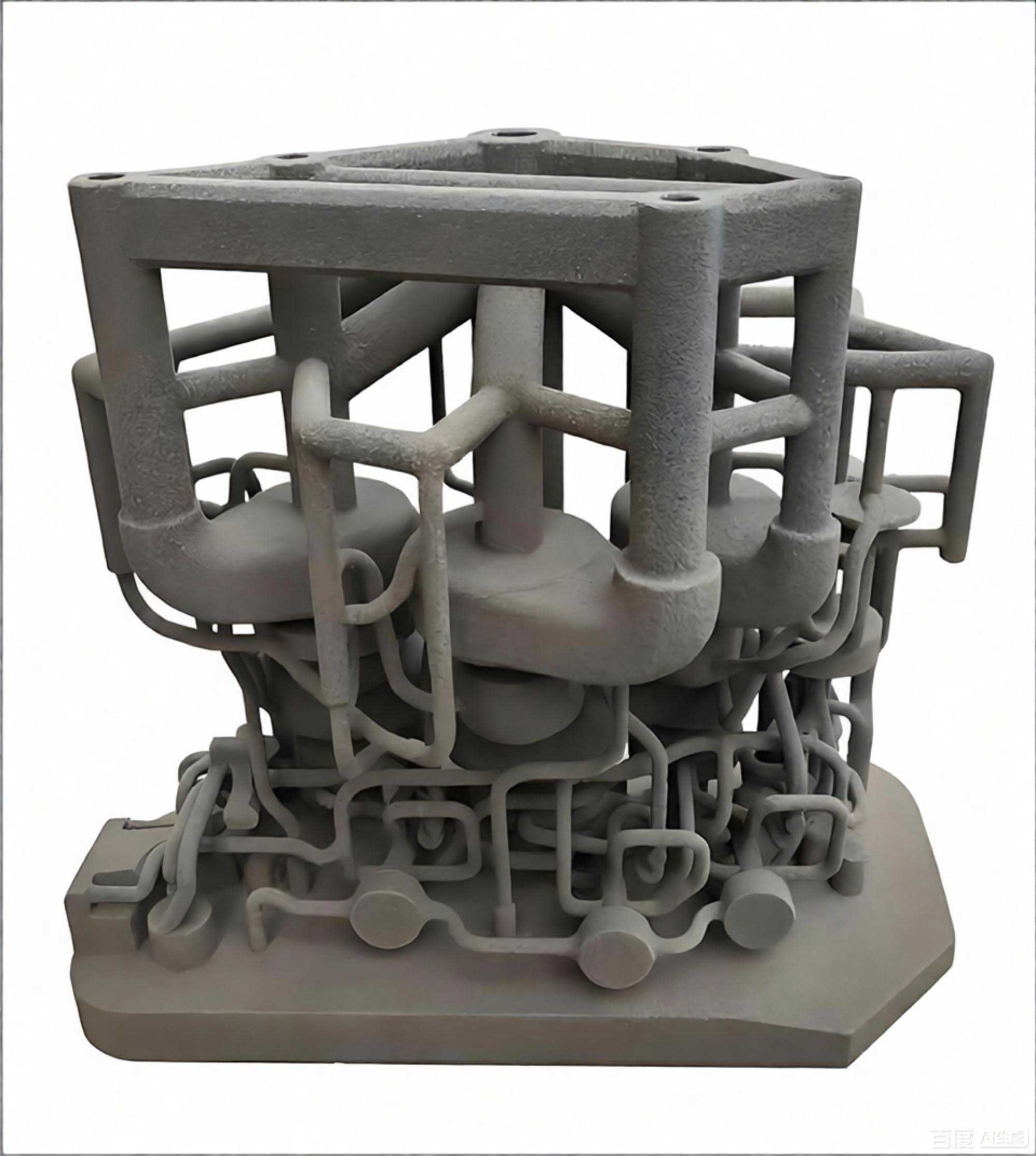
In my research, I focused on the optimization of steel castings manufactured through 3D sand printing. 3D sand printing is an indirect additive manufacturing technique that has revolutionized traditional sand casting by enabling complex geometries, reducing tooling costs, and shortening lead times. Unlike conventional mold-making processes, 3D sand printing builds sand molds layer by layer directly from CAD data, which allows me to design gating systems and internal cavities that would be impossible or extremely expensive to produce with traditional pattern-based methods. This study integrates response surface methodology (RSM) for parameter optimization and numerical simulation using ProCAST for casting process design. The central goal is to improve the quality of a natural gas meter housing made of 316 stainless steel by minimizing casting defects and enhancing the mechanical performance of the printed sand mold.
Throughout this paper, I repeatedly emphasize the role of 3d sand printing in enabling flexible and efficient foundry practices. The technology is particularly beneficial for small-batch and highly customized components, where the cost of a physical pattern cannot be justified. By using a binder jetting approach, the printer selectively deposits furan resin onto a bed of silica sand pre-mixed with a curing agent. After layer-by-layer consolidation, the mold is cured naturally, then cleaned and ready for pouring. The main issues I encountered are the trade-off between mold strength and gas evolution, as well as the need for a robust gating system to avoid shrinkage porosity and misruns. To solve these problems, I designed a series of experiments and simulations.
Experimental Materials and Methods
For all experiments, I used a special silica sand specifically developed for 3d sand printing. The sand had a uniform grain size, low acid demand, and low thermal expansion, which ensured smooth spreading and stable mold dimensions. Table 1 lists the key properties of the raw sand.
| Property | Value |
|---|---|
| Moisture content (%) | 0.08 |
| Mud content (%) | 0.12 |
| Acid demand (%) | 3.1 |
| Ignition loss (%) | 0.15 |
| Bulk density (g/cm³) | 1.47 |
The binder used was furan resin, which provides excellent self-hardening characteristics and good collapsibility. Table 2 shows the main parameters of the furan resin.
| Parameter | Value |
|---|---|
| Water content (%) | 3.47 |
| Nitrogen content (%) | 0.02 |
| Density (g/cm³) | 1.151 |
| Viscosity at 20°C (MPa·s) | 19 |
| Free formaldehyde (%) | 0.09 |
As the curing agent, I used p-toluenesulfonic acid with a low density to ensure homogeneous mixing. The total acidity was 0.08%, and the viscosity at 20°C was 0.15 MPa·s. The printing equipment was an HX1000 3D sand printer with a build volume of 1000 mm × 800 mm × 600 mm. The machine allowed me to set the layer thickness from 0.25 to 0.4 mm, the resin content from 0.5% to 2% by weight of sand, and the curing agent content from 2‰ to 4‰ by weight of sand. During printing, the sand and curing agent were mixed in a hopper, then spread by a roller, and the printhead selectively deposited furan resin droplets to bond the sand particles. After completion, the mold was left to cure at room temperature for 24 hours before testing.
For tensile strength measurements, I printed standard dog-bone specimens according to GB/T 2684-2009. The specimens were tested on an XQY-II intelligent sand strength machine. For gas evolution, I used a GET-III intelligent gas evolution tester. Powder samples of 1.00 g were taken from fractured specimens and heated to 850°C, and the volume of evolved gas was recorded. Each measurement was repeated six times, and the average was reported.
Single-Factor Experiments and Response Surface Optimization
To determine the center points for response surface design, I first performed single-factor experiments. I fixed the printing speed, ink jetting rate, ambient temperature at 25°C, and curing time at 24 h. For layer thickness experiments, I used a resin content of 2% and curing agent content of 3.5‰. The results showed that as layer thickness increased from 0.3 mm to 0.4 mm, tensile strength decreased from 0.993 MPa to 0.626 MPa, while gas evolution decreased from 12.9 mL/g to 10.8 mL/g. The decrease in strength is attributed to fewer printed layers and lower overall resin content in the thicker layers. For resin content experiments, I fixed layer thickness at 0.35 mm and curing agent at 3.5‰. As resin increased from 1% to 2%, tensile strength rose from 0.714 MPa to 1.011 MPa, and gas evolution increased from 10.1 mL/g to 11.9 mL/g. For curing agent experiments, with layer thickness 0.35 mm and resin 1.5%, tensile strength increased from 0.715 MPa to 0.731 MPa when curing agent rose from 3‰ to 4‰, while gas evolution increased significantly from 8.3 mL/g to 12.2 mL/g. Based on these results, I selected the center values: layer thickness 0.35 mm, resin content 1.5%, and curing agent content 3.5‰.
I then conducted a three-factor, three-level Box-Behnken design using Design-Expert 10 software. The factors and levels are listed in Table 3.
| Factor | -1 | 0 | 1 |
|---|---|---|---|
| Layer thickness (mm) | 0.3 | 0.35 | 0.4 |
| Resin content (%) | 1 | 1.5 | 2 |
| Curing agent content (‰) | 3 | 3.5 | 4 |
The complete experimental design and measured responses are shown in Table 4.
| Run | A: Layer (mm) | B: Resin (%) | C: Curing agent (‰) | Tensile strength (MPa) | Gas evolution (mL/g) |
|---|---|---|---|---|---|
| 1 | -1 | -1 | 0 | 0.682 | 10.8 |
| 2 | 1 | -1 | 0 | 0.535 | 9.4 |
| 3 | -1 | 1 | 0 | 1.071 | 13.6 |
| 4 | 1 | 1 | 0 | 0.518 | 12.3 |
| 5 | -1 | 0 | -1 | 0.712 | 8.8 |
| 6 | 1 | 0 | -1 | 0.533 | 7.8 |
| 7 | -1 | 0 | 1 | 1.011 | 14.2 |
| 8 | 1 | 0 | 1 | 0.468 | 11.9 |
| 9 | 0 | -1 | -1 | 0.426 | 8.6 |
| 10 | 0 | 1 | -1 | 0.586 | 8.1 |
| 11 | 0 | -1 | 1 | 0.679 | 11.8 |
| 12 | 0 | 0 | 0 | 0.754 | 9.9 |
| 13 | 0 | 0 | 0 | 0.714 | 11.9 |
| 14 | 0 | 0 | 0 | 0.634 | 12.7 |
| 15 | 0 | 0 | 0 | 0.628 | 11.9 |
| 16 | 0 | 0 | 0 | 0.681 | 12.4 |
| 17 | 0 | 0 | 0 | 0.637 | 11.5 |
Regression Model for Tensile Strength
Using the least squares method, I obtained the following quadratic response surface model for tensile strength (Y₁):
$$ Y_1 = -0.66 – 0.18A + 0.076B + 0.082C – 0.10AB – 0.091AC – 0.021BC + 0.056A^2 – 0.014B^2 – 0.034C^2 $$
The analysis of variance (ANOVA) for this model is presented in Table 5.
| Source | Sum of squares | df | Mean square | F value | P value | Significance |
|---|---|---|---|---|---|---|
| Model | 0.45 | 9 | 0.050 | 28.01 | 0.0001 | ** |
| A | 0.25 | 1 | 0.25 | 142.67 | <0.0001 | ** |
| B | 0.046 | 1 | 0.046 | 26.00 | 0.0014 | ** |
| C | 0.054 | 1 | 0.054 | 30.27 | 0.0009 | ** |
| AB | 0.041 | 1 | 0.041 | 23.26 | 0.0019 | ** |
| AC | 0.033 | 1 | 0.033 | 18.70 | 0.0035 | ** |
| BC | 1.81×10⁻⁴ | 1 | 1.81×10⁻⁴ | 1.02 | 0.3463 | – |
| A² | 0.016 | 1 | 0.013 | 7.49 | 0.0291 | – |
| B² | 7.82×10⁻⁴ | 1 | 1.81×10⁻⁴ | 1.12 | 0.5278 | – |
| C² | 4.90×10⁻⁴ | 1 | 4.90×10⁻³ | 2.77 | 0.1401 | – |
| Residual | 0.012 | 7 | 1.77×10⁻³ | |||
| Lack of fit | 6.77×10⁻³ | 3 | 2.26×10⁻³ | 1.61 | 0.3212 | |
| Pure error | 5.62×10⁻³ | 4 | 1.41×10⁻⁴ | |||
| Total | 0.46 | 16 |
Note: ** highly significant (P < 0.01); * significant (P < 0.05). The coefficient of determination R² = 0.9730 and adjusted R² = 0.9382, indicating excellent fit. From the F values, the order of influence on tensile strength is layer thickness (A) > curing agent content (C) > resin content (B).
Regression Model for Gas Evolution
For gas evolution (Y₂), the regression model is:
$$ Y_2 = 10.72 – 1.08A + 1.21B + 0.36C + 0.075AB + 0.025AC – 1.05BC – 0.54A^2 + 0.44B^2 – 0.61C^2 $$
The ANOVA results are shown in Table 6.
| Source | Sum of squares | df | Mean square | F value | P value | Significance |
|---|---|---|---|---|---|---|
| Model | 30.02 | 9 | 3.34 | 68.57 | < 0.0001 | ** |
| A | 9.24 | 1 | 9.24 | 190.06 | < 0.0001 | ** |
| B | 11.76 | 1 | 11.76 | 241.79 | < 0.0001 | ** |
| C | 1.05 | 1 | 1.05 | 21.61 | 0.0023 | ** |
| AB | 0.023 | 1 | 0.023 | 0.46 | 0.5183 | – |
| AC | 2.50×10⁻³ | 1 | 2.50×10⁻³ | 0.051 | 0.8271 | – |
| BC | 4.41 | 1 | 4.41 | 90.66 | < 0.0001 | ** |
| A² | 1.21 | 1 | 1.21 | 24.78 | 0.0016 | * |
| B² | 0.82 | 1 | 0.82 | 16.76 | 0.0046 | * |
| C² | 1.57 | 1 | 1.57 | 32.21 | 0.0008 | ** |
| Residual | 0.34 | 7 | 0.049 | |||
| Lack of fit | 0.23 | 3 | 0.077 | 2.87 | 0.1673 | |
| Pure error | 0.11 | 4 | 0.027 | |||
| Total | 30.86 | 16 |
The model R² = 0.9888, adjusted R² = 0.9744, confirming very good prediction accuracy. The order of influence on gas evolution is resin content (B) > layer thickness (A) > curing agent content (C). The interaction BC is highly significant, meaning resin content and curing agent content collectively affect gas evolution.
Optimal Parameters and Verification
Using numerical optimization in Design-Expert, I set the objectives to maximize tensile strength and minimize gas evolution. The suggested optimum was a layer thickness of 0.3 mm, resin content of 1.629%, and curing agent content of 4‰. Considering practical adjustability, I selected the following optimum parameters: layer thickness = 0.3 mm, resin content = 1.6%, and curing agent content = 4‰. I then printed four additional specimens to verify the model predictions. The results are shown in Table 7.
| No. | Layer (mm) | Resin (%) | Curing agent (‰) | Tensile strength (MPa) | Gas evolution (mL/g) |
|---|---|---|---|---|---|
| 1 | 0.3 | 1.6 | 4 | 1.063 | 11.0 |
| 2 | 0.3 | 1.6 | 4 | 1.049 | 11.3 |
| 3 | 0.3 | 1.6 | 4 | 1.050 | 11.2 |
| 4 | 0.3 | 1.6 | 4 | 1.058 | 10.9 |
| Average | 1.055 | 11.1 |
The measured average tensile strength was 1.055 MPa and gas evolution was 11.1 mL/g, which are close to the predicted values. This confirms that the response surface models are reliable for optimizing 3d sand printing parameters.
Casting Process Design for a Complex Steel Part
After optimizing the sand mold parameters, I proceeded to design the casting process for a natural gas meter housing made of 316 stainless steel. The part is a thin-walled cylindrical shell with a central partition wall, several bosses, and a flange. The wall thickness varies from 4 mm to 7 mm, with a maximum thickness of 15 mm at the flange. Because of the complexity and thin sections, 3d sand printing is an ideal manufacturing method because it avoids the need for a separate core package and minimizes assembly errors. The casting material is 0Cr17Ni12Mo2 (316 stainless steel) with the chemical composition shown in Table 8.
| Element | C | Si | Mn | P | S | Ni | Cr | Mo |
|---|---|---|---|---|---|---|---|---|
| Content (%) | ≤0.08 | ≤1.00 | ≤2.00 | ≤0.035 | ≤0.03 | 10-14 | 16.0-18.5 | 2.0-3.0 |
Key mechanical properties of this steel are: ultimate tensile strength ≥ 520 MPa, yield strength ≥ 205 MPa, elongation ≥ 40%, density 7.98 g/cm³, and specific heat capacity 0.502 J/(g·K) at 20°C. The pouring temperature was set to 1560°C to account for heat loss during filling.
Gating System Design
I chose a closed-open gating system to prevent slag entrapment and ensure smooth filling. Because 3d sand printing permits arbitrary geometries, I designed circular-cross-section runners, which reduce heat loss and improve metal flow compared to trapezoidal channels. The sprue, runner, and ingate area ratio was determined as A_sprue : A_runner : A_ingate = 11 : 9 : 10. Using the section-ratio method, the ingate area was calculated from:
$$ A_{\text{ingate}} = \frac{G}{\mu \rho \tau \sqrt{2g H_p}} $$
where \(G\) is the total mass of molten metal, \(\rho\) is the metal density, \(\tau\) is the filling time, \(\mu\) is the flow coefficient, and \(H_p\) is the average pressure head. After calculation and adjustment, the final radii were: sprue radius 15 mm, runner radius 12 mm, and ingate radius 13 mm. The pouring time was about 4 seconds, and the total metal mass required was 4.237 kg.
I designed three gating configurations to evaluate the effect of filling direction on defect formation. The first is a single-side ingate scheme (Scheme A), the second is a bilateral ingate scheme (Scheme B), and the third is a reverse bilateral ingate scheme (Scheme C). These schemes represent different positions of the ingates relative to the part geometry. Since the part has a flange on one side and a blind boss on the other, the placement of ingates strongly influences the flow pattern and temperature distribution.
Numerical Simulation Setup
For simulation, I used ProCAST, a finite-element solver for casting processes. I built the 3D CAD model of the part with gating systems in NX 12.0 and exported it as a Parasolid file. After importing into ProCAST, I generated surface meshes with a target size of 3 mm for the casting and 4 mm for the mold. I refined the mesh in thin-walled regions and complex fillets to ensure accurate heat transfer and fluid flow. The mesh generation is shown conceptually by the different zones of the model.
Material properties for the steel were computed in ProCAST based on the chemical composition. The liquidus temperature was 1505°C, and the pouring temperature was set to 1560°C. The sand mold material was defined as furan-resin-bonded sand with temperature-dependent thermal properties. The initial temperature of the sand was 25°C. Heat transfer coefficients were set as follows: casting–mold interface: 1000 W·m⁻²·K⁻¹; casting–chill interface: 2000 W·m⁻²·K⁻¹; and mold–air interface: free convection. I set the filling limit to 100% and the flow rate was calculated automatically by the solver.
Filling and Solidification Simulation Results
Filling Process Analysis
For Scheme A (single-side ingate), the molten metal entered the cavity quickly but preferentially on one side. At 1 s, the metal had filled only the right half of the mold, with a low-velocity zone near the boss. At 2 s, the metal covered about two-thirds of the cavity, but there were stagnant regions in the middle that could lead to cold shuts. At 3 s, the metal surface was uneven between the left and right sides. At 4 s, the cavity was full, but the flow pattern was unstable.
For Scheme B (bilateral ingate), the metal flow was more symmetrical. At 2 s, the two streams met in the lower part of the mold with a small turbulent zone, but the liquid level rose uniformly. At 3 s, the metal filled the inner cavity and the thin walls at a speed of about 0.5–0.8 m/s. At 4 s, the entire part was filled smoothly, without any misruns or cold shuts. This scheme promoted consistent solidification because both sides filled at nearly the same rate.
For Scheme C (reverse bilateral ingate), the metal filled the flange area first at 1 s. At 2 s, the flange was completely filled, but the flow velocity in the lower boss region varied from 0.2 to 0.6 m/s across the same section, indicating potential turbulence and oxide entrapment. At 4 s, the part was still not completely filled in the upper thin sections, suggesting that this scheme has the highest risk of misrun.
Solidification and Temperature Field Analysis
Scheme A solidified rapidly but non-uniformly. The central partition and flange solidified first, while the lower thin plate formed an isolated liquid region that remained hot until 175 s. This isolated liquid is a classic source of shrinkage porosity and cold shuts.
Scheme B exhibited progressive solidification. The thinnest sections near the center solidified in about 9 s, while the flange and ingate areas required about 71 s. The temperature gradients were orderly, and no isolated liquid pools were observed. At 147 s, most of the part had solidified except for some thick regions near the ingates that were fed by the sprue. This directional solidification is beneficial for defect reduction.
Scheme C solidified slowly and unevenly. The lower boss right side took about 100 s to solidify, creating a long-lasting hot spot. The reverse flow caused irregular temperature distribution, and at 143 s, the sprue-side walls were still at 1260°C, whereas Scheme B had cooled to about 1160°C. Such hot spots increase the likelihood of shrinkage defects.
Defect Prediction
Using the Niyama criterion, I predicted shrinkage porosity locations. Scheme A produced a total shrinkage porosity volume of 0.559 cc, mainly in the lower thick wall and flange. Scheme B produced 0.391 cc, concentrated at the flange and some scattered small pores. Scheme C produced 0.499 cc, distributed on both sides of the flange and center. Table 9 summarizes the defect parameters.
| Parameter | Scheme A | Scheme B | Scheme C |
|---|---|---|---|
| Total volume (cc) | 3.533 | 3.445 | 2.476 |
| Shrinkage porosity volume (cc) | 0.559 | 0.391 | 0.499 |
| Density (g/cc) | 1.20 | 1.20 | 1.20 |
| Weight (mg) | 0.671 | 0.469 | 0.599 |
Based on filling uniformity, solidification sequence, and defect volume, I selected Scheme B as the optimal base design. Its defects are concentrated and can be effectively eliminated by adding risers and chills.
Process Optimization of the Selected Scheme
Riser Design
To eliminate the concentrated shrinkage in the flange area, I designed two open-top risers placed on top of the flange. Using the modulus method, I calculated the riser modulus as:
$$ M = \frac{V}{A} $$
where V is the riser volume and A is the cooling surface area. The calculated modulus was 3.8 mm. Using the thermal circle method, I determined a riser diameter of 29 mm and a riser height of 35 mm, with a 4 mm fillet radius at both the top and bottom. The risers were designed with a neck to facilitate feeding and easy removal. Figure below illustrates the optimized layout (not shown here), but the final riser arrangement helped to feed the flange hot spots and significantly reduce porosity.
Chill Placement
A steel chill was placed under the lower thick-wall section of the part, where the original simulation showed a slow solidifying region. The chill dimensions were designed according to the local geometry. The chill accelerates cooling in that thick section, promoting a bottom-to-top directional solidification. The presence of the chill also reduces the local thermal gradient and minimizes the risk of hot tears.
Casting Process Parameters
According to the casting process manual, I assigned the following parameters. The dimensional tolerance grade was CT13 with a tolerance size of 10 mm. The weight tolerance grade was M13, corresponding to a weight tolerance of 24%. The machining allowance was selected as 9 mm. For the flange area, I added a process correction of 2 mm to account for the higher risk of expansion or distortion. These parameters were applied to the final model before simulation.
Numerical Simulation of the Optimized Process
After adding risers and chill, I reran the ProCAST simulation. The material definitions and boundary conditions are summarized in Table 10.
| Name | Type | Material | Initial temperature (°C) |
|---|---|---|---|
| PART (casting + risers) | Alloy | 316 stainless steel | 1560 |
| SAND MOLD | Mold | Furan resin sand | 25 |
| CHILL | Mold | Iron | 25 |
The optimized filling process showed that the metal entered the cavity at a velocity of about 0.7 m/s and filled the lower thick section first. Compared to the original scheme, the lower section no longer exhibited slow filling. The liquid level rose uniformly without large velocity variations. The entire cavity was filled in 4 seconds without any misruns.
The solidification sequence changed from the original. At 17 s, the lower thickened region under the influence of the chill was already solidifying, while the thin walls also solidified quickly. At 67 s, the solidification front moved upward symmetrically. At 147 s, the entire casting had solidified following a bottom-to-top directional pattern. No isolated liquid pools remained. The risers remained liquid longer than the casting, allowing them to feed the flange areas.
The defect analysis showed that the shrinkage porosity inside the casting was nearly eliminated. The remaining porosity inside the casting was only 0.0008 cc, while the risers contained 0.073 cc of porosity. Compared to the unoptimized Scheme B, which had 0.391 cc of shrinkage porosity, the optimized process achieved a 99.8% reduction in internal porosity. The defects outside the casting are acceptable and can be removed with the risers.
These simulation results demonstrate that the optimized casting process, combined with 3d sand printing, is capable of producing sound steel castings with complex thin-walled geometry. The use of optimized sand mold parameters ensures adequate mold strength and low gas evolution, while the carefully designed gating and feeding system minimizes defects.
Conclusion
In this research, I successfully optimized the process parameters for 3d sand printing of furan resin-bonded sand molds and designed a robust casting process for a 316 stainless steel natural gas meter housing. The key findings are summarized as follows:
- Through single-factor experiments and response surface methodology, I obtained the optimum 3d sand printing parameters: layer thickness 0.3 mm, resin content 1.6%, and curing agent content 4‰. The verification experiments produced a tensile strength of 1.055 MPa and a gas evolution of 11.1 mL/g, which closely matched the model predictions.
- For tensile strength, the significance order of the factors was layer thickness > curing agent content > resin content. For gas evolution, the order was resin content > layer thickness > curing agent content. The strongest interaction for gas evolution was between resin content and curing agent content.
- I designed a closed-open gating system with circular runners and a sprue:runner:ingate ratio of 11:9:10. Among three gating schemes, the bilateral ingate scheme (Scheme B) provided the most stable filling and progressive solidification, with a shrinkage porosity volume of 0.391 cc.
- By adding two open-top risers and a steel chill, I converted the solidification mode into a directional bottom-to-top sequence. The optimized simulation showed that the internal porosity was reduced to 0.0008 cc, while the risers contained 0.073 cc of porosity, representing a significant improvement over the unoptimized process.
- The combination of 3d sand printing and numerical simulation provides a powerful approach for producing high-quality complex steel castings with reduced lead time and cost.
In summary, 3d sand printing not only enables the fabrication of intricate mold geometries but also allows the foundry engineer to iterate quickly on gating designs. The response surface optimization demonstrates that careful control of printing parameters is essential to achieve the required mold strength and minimum gas generation. The simulation-based design ensures that the casting solidifies in a directional manner, thereby minimizing defects. This integrated methodology can be extended to other cast alloys and complex components, making 3d sand printing a key enabler for smart and green casting manufacturing.